Demo: dark mode

David Hodge

Overview

This article will demonstrate each wrapper function.

library(dplyr)
#> Error in get(paste0(generic, ".", class), envir = get_method_env()) : 
#>   object 'type_sum.accel' not found
library(ggplot2)
library(scales)
library(ggblanket)
library(palmerpenguins)

set_blanket(
  mode = dark_mode_r(), 
  text_colour = darkness[1],
  reference_colour = darkness[1],
  col_palette_d = c(teal, orange, purple, red, pink, navy),
  col_palette_c = viridis::mako(n = 9),
  col_palette_o = scales::pal_viridis(option = "G"),
)

penguins2 <- penguins |> 
  labelled::set_variable_labels(
    bill_length_mm = "Bill length (mm)",
    bill_depth_mm = "Bill depth (mm)",
    flipper_length_mm = "Flipper length (mm)",
    body_mass_g = "Body mass (g)",
  ) |> 
  mutate(sex = factor(sex, labels = c("Female", "Male"))) |>
  tidyr::drop_na(sex)

experiment <- data.frame(
  trt = factor(c(1, 1, 2, 2)),
  resp = c(1, 5, 3, 4),
  group = factor(c(1, 2, 1, 2)),
  upper = c(1.1, 5.3, 3.3, 4.2),
  lower = c(0.8, 4.6, 2.4, 3.6)) |>
  labelled::set_variable_labels(
    trt = "Treatment", 
    resp = "Response"
  )

gg_area

economics |>
  gg_area(
    x = date,
    y = unemploy,
    y_label = "Unemployment",
  )

gg_bar

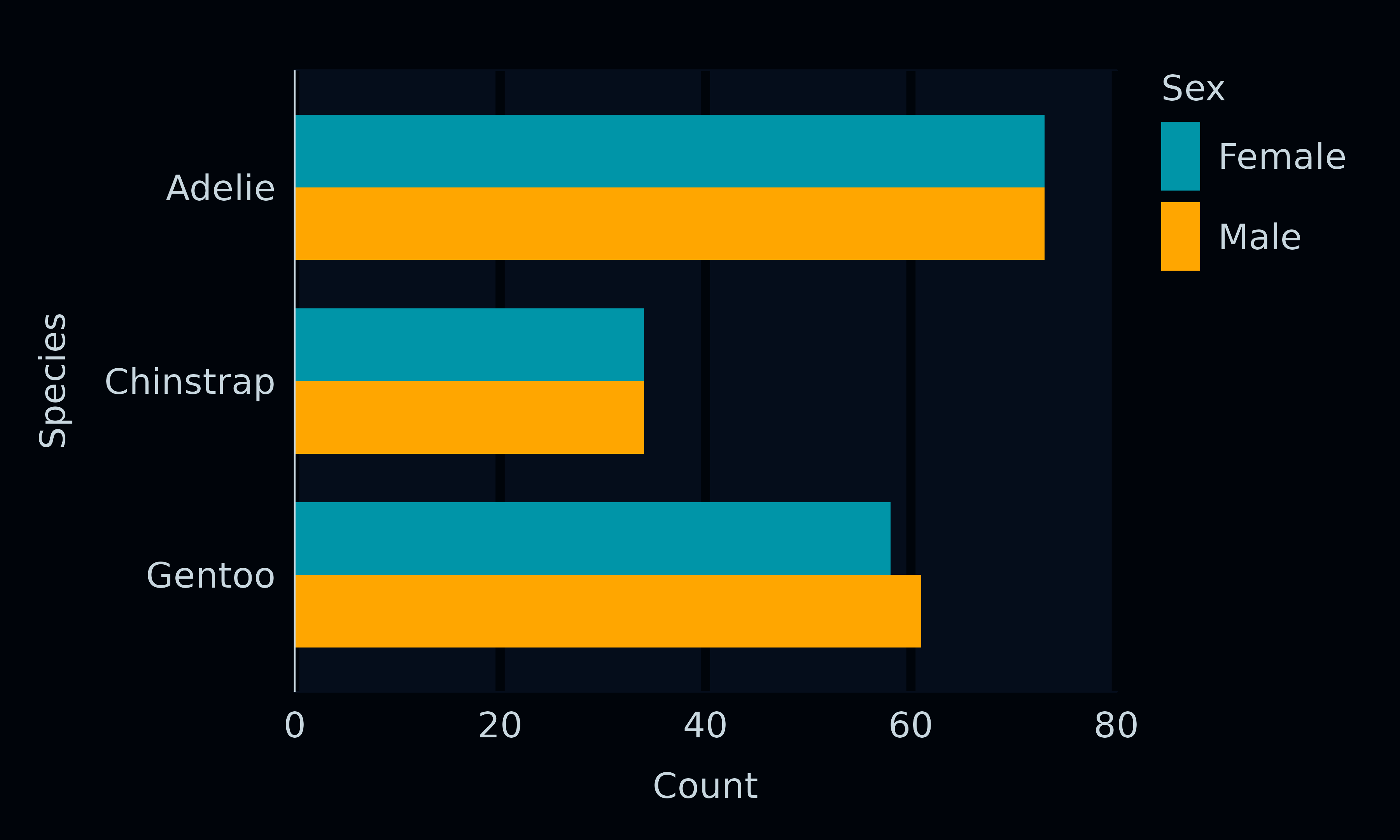
penguins2 |>
  gg_bar(
    position = position_dodge(preserve = "single"),
    y = species,
    col = sex,
    width = 0.75,
  )

gg_bin_2d

diamonds |>
  gg_bin_2d(
    x = carat,
    y = price,
  )

gg_boxplot

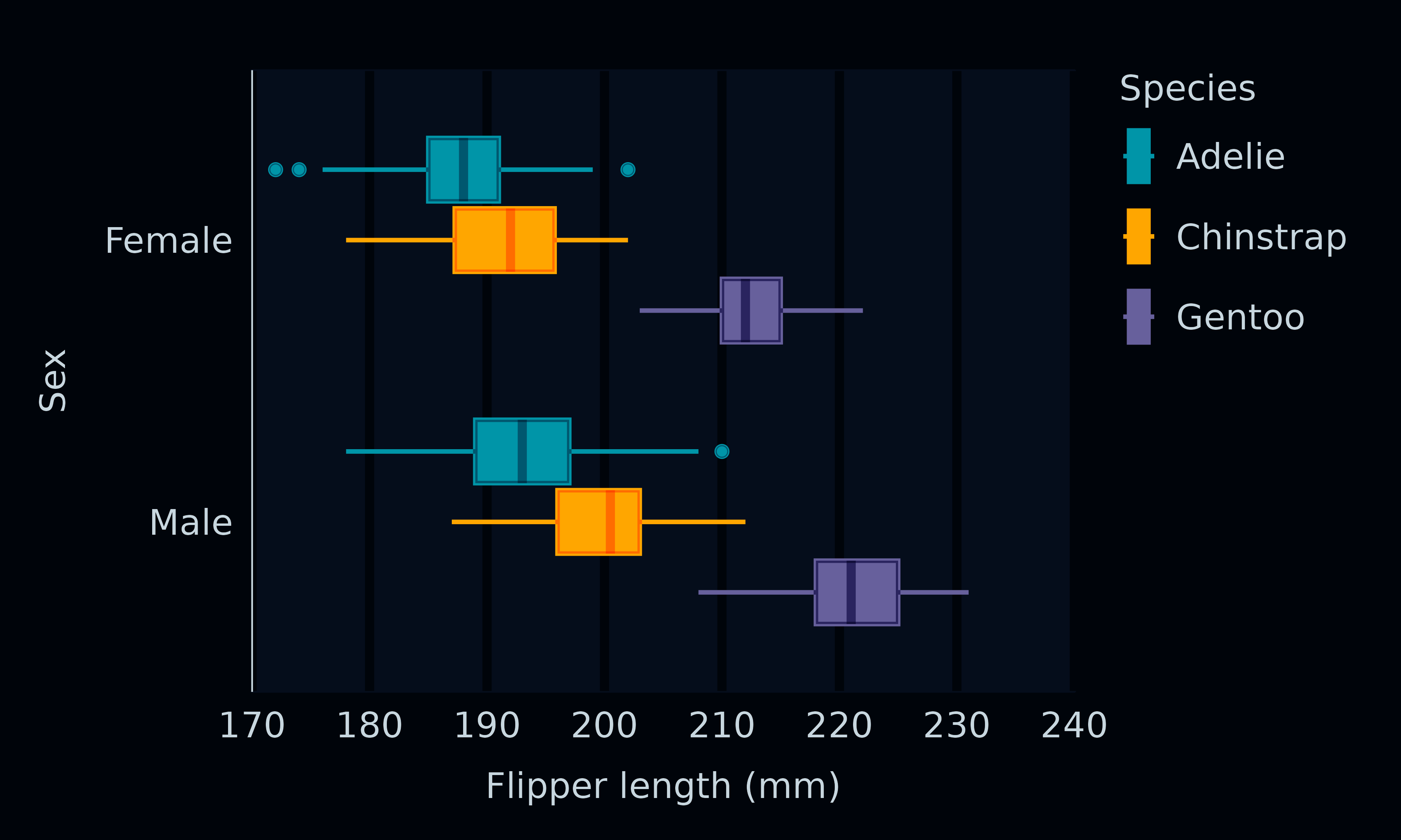
penguins2 |>
  gg_boxplot(
    x = flipper_length_mm,
    y = sex,
    col = species,
    blend = "multiply",
  )

gg_col

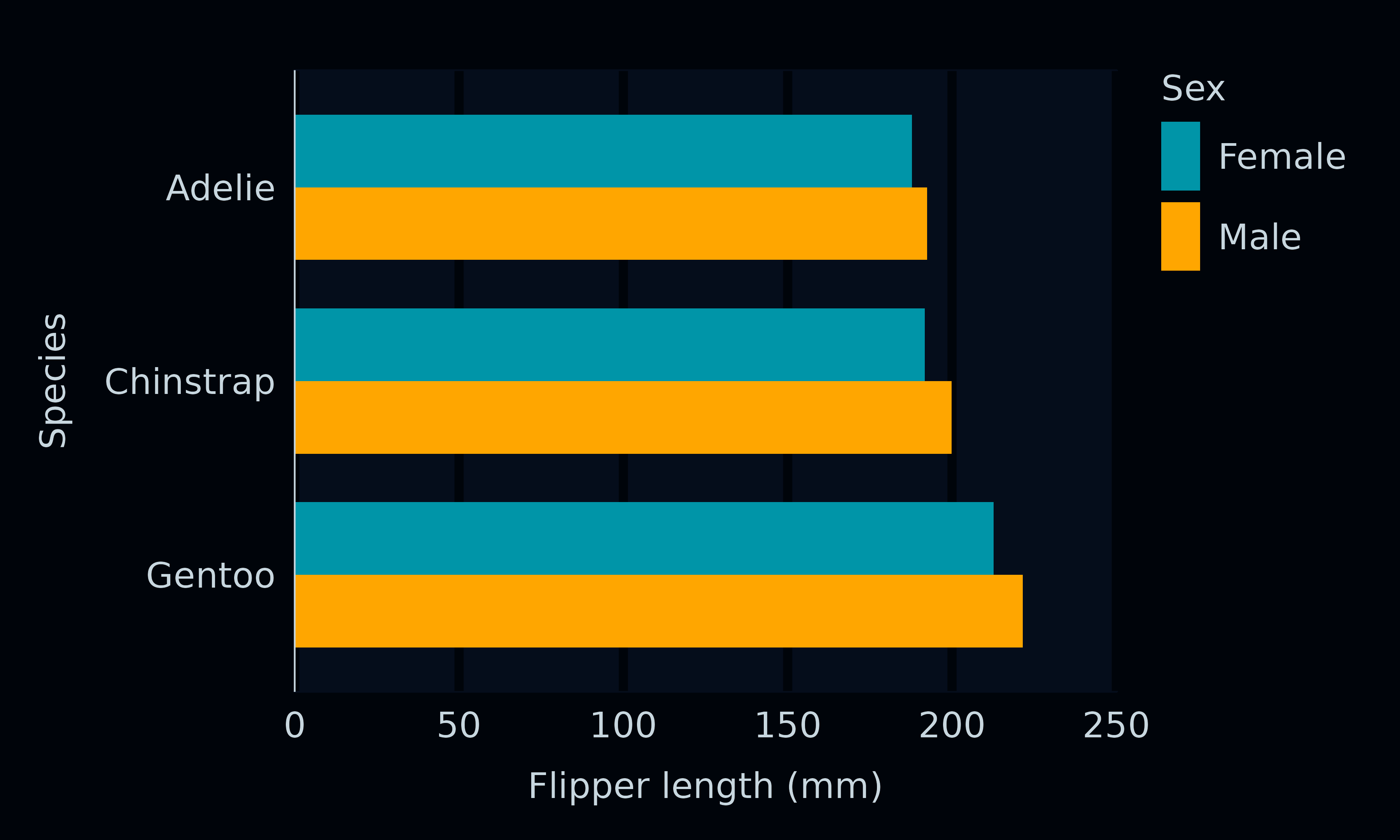
penguins2 |>
  group_by(sex, species) |>
  summarise(across(flipper_length_mm, \(x) mean(x, na.rm = TRUE))) |>
  labelled::copy_labels_from(penguins2) |>
  gg_col(
    position = position_dodge(preserve = "single"),
    x = flipper_length_mm,
    y = species,
    col = sex,
    width = 0.75,
  )

gg_contour

faithfuld |>
 gg_contour(
   x = waiting,
   y = eruptions,
   z = density,
  )

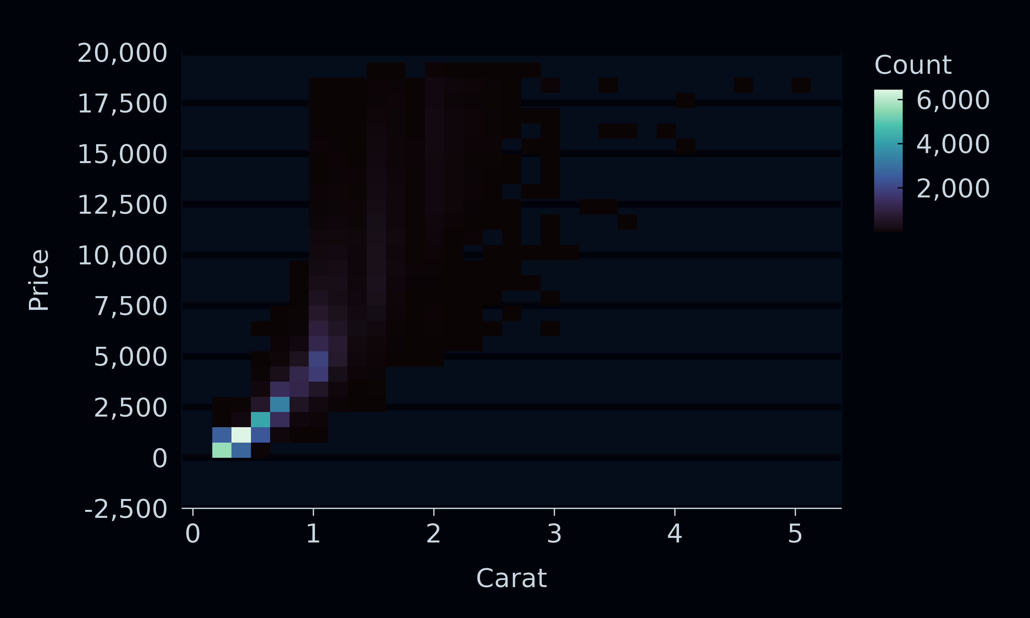
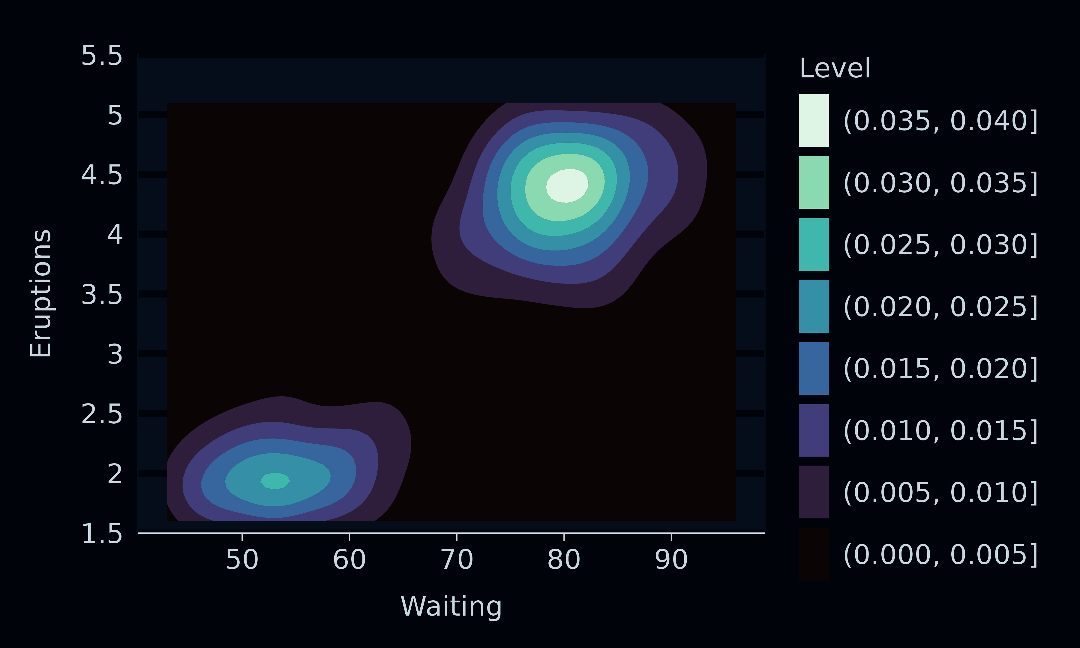
gg_contour_filled

faithfuld |>
 gg_contour_filled(
   x = waiting,
   y = eruptions,
   z = density,
   bins = 8,
  )

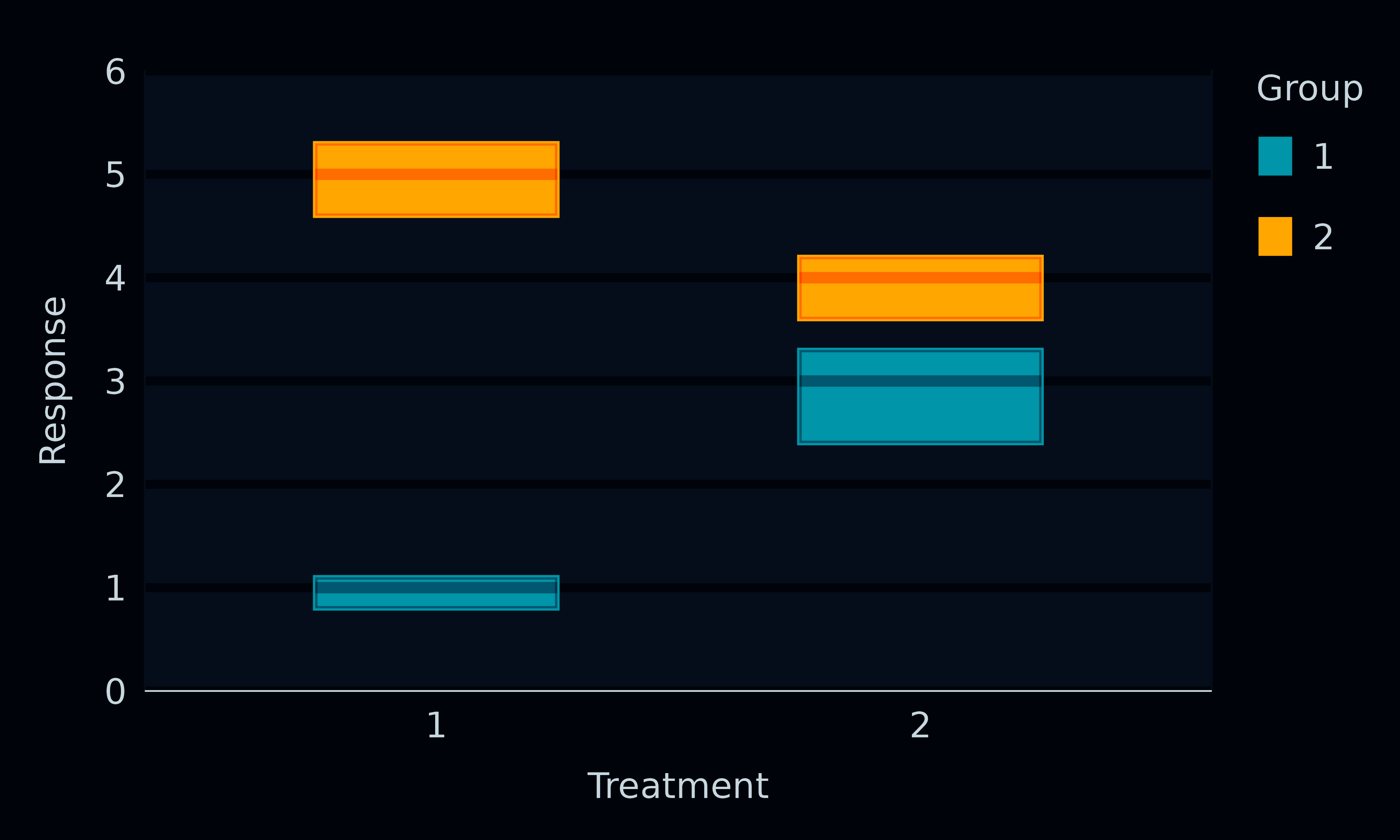
gg_crossbar

experiment |>
  gg_crossbar(
    x = trt,
    y = resp,
    ymin = lower,
    ymax = upper,
    col = group,
    width = 0.5,
    y_expand_limits = 0,
    blend = "multiply",
  )

gg_density

penguins2 |>
  gg_density(
    x = flipper_length_mm,
    col = species,
    blend = "multiply",
  )

gg_density_2d

faithful |>
  gg_density_2d(
    x = waiting,
    y = eruptions,
    bins = 8,
    contour = TRUE,
  )

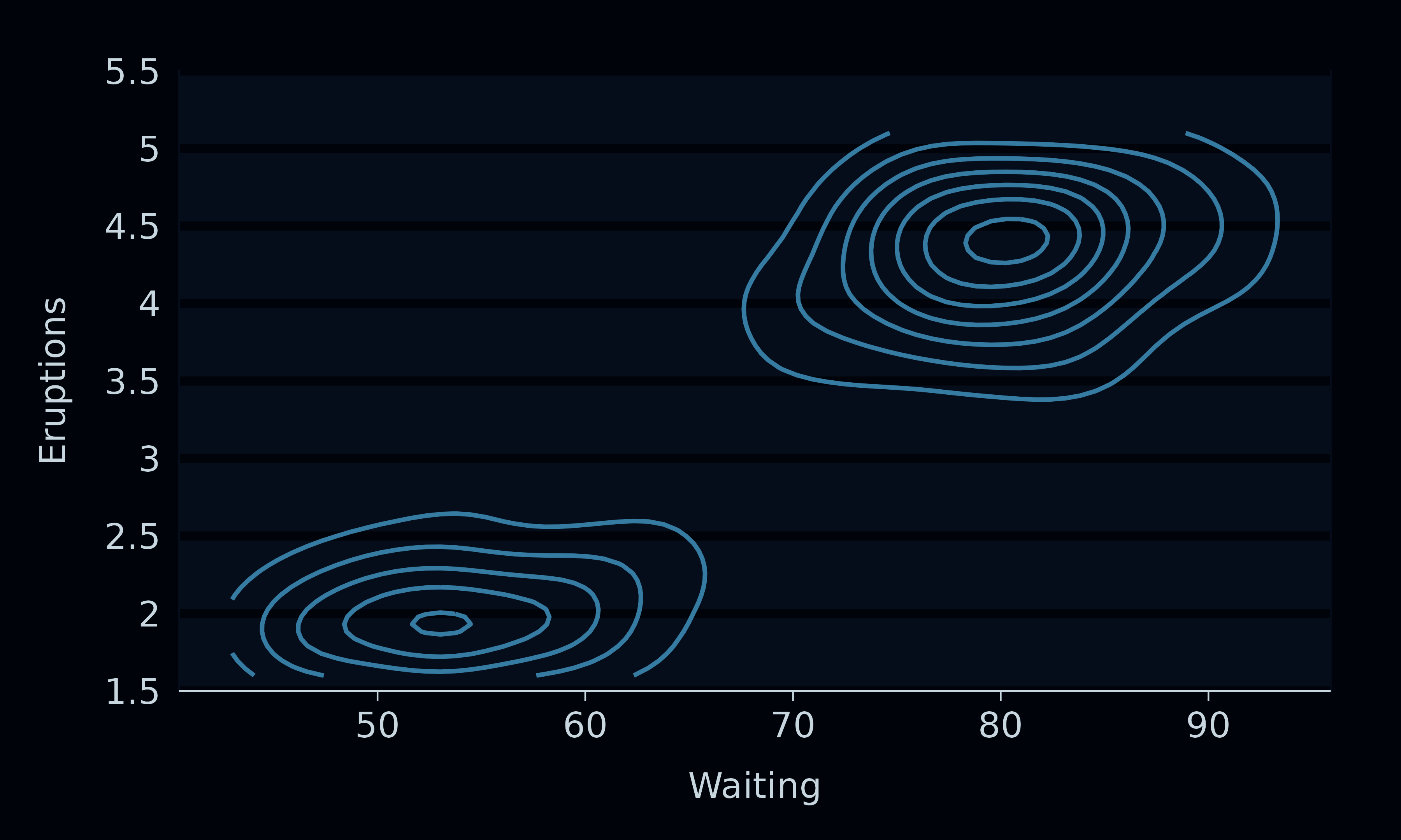
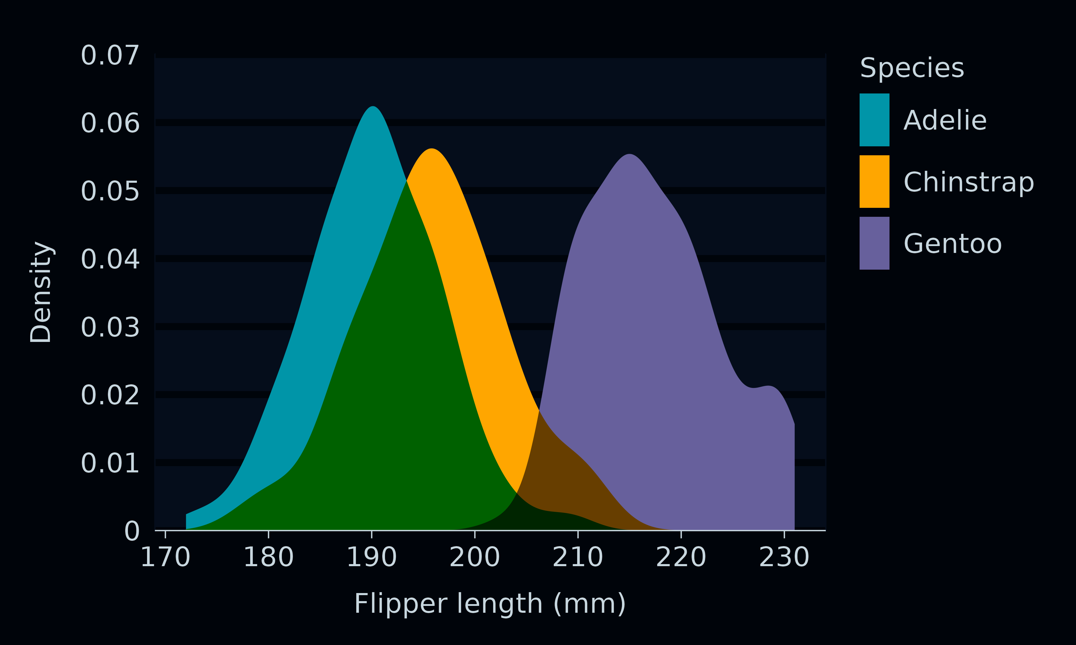
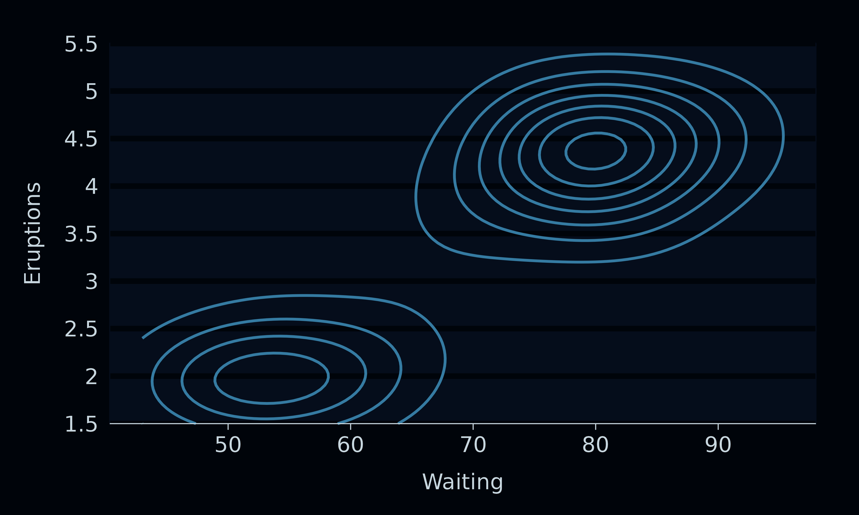
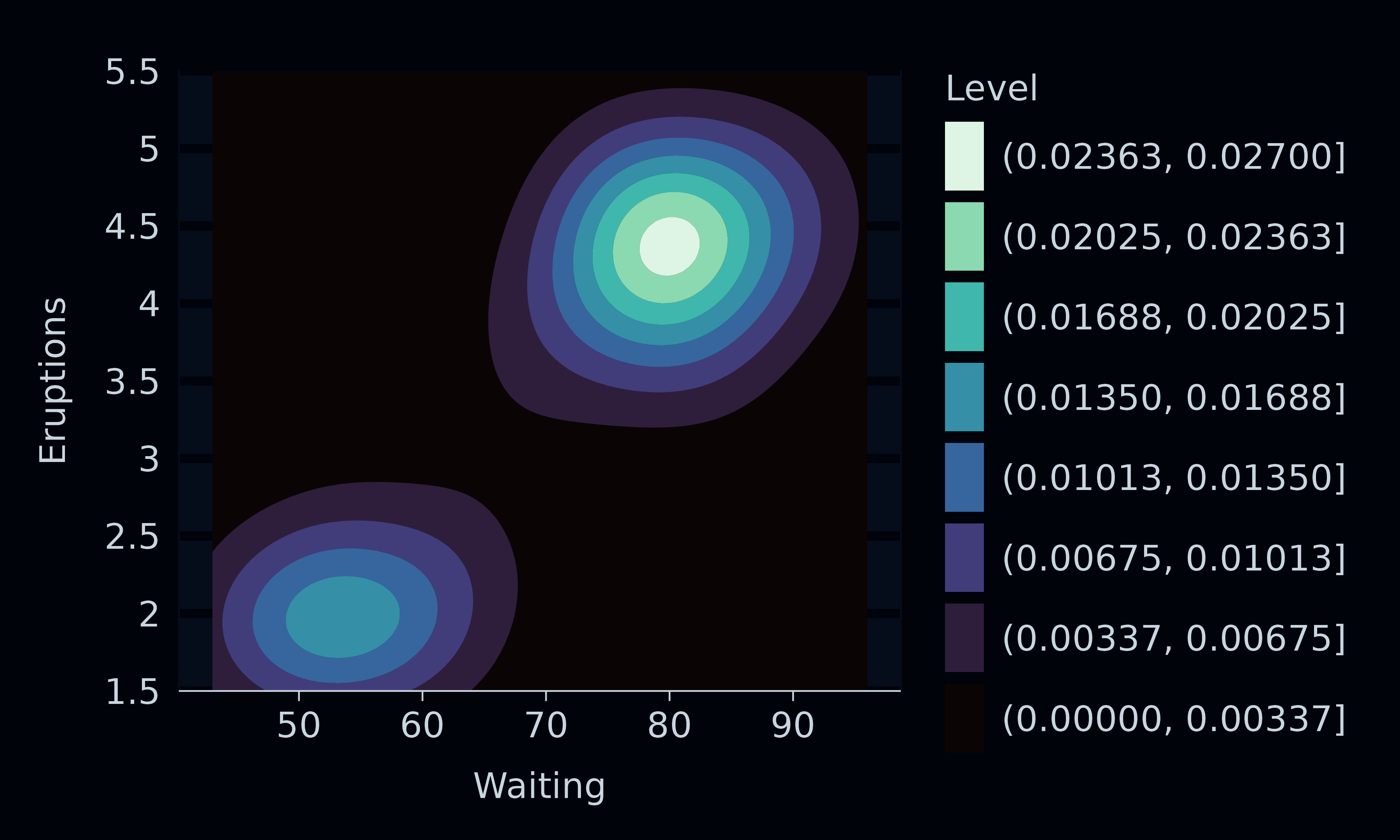
gg_density_2d_filled

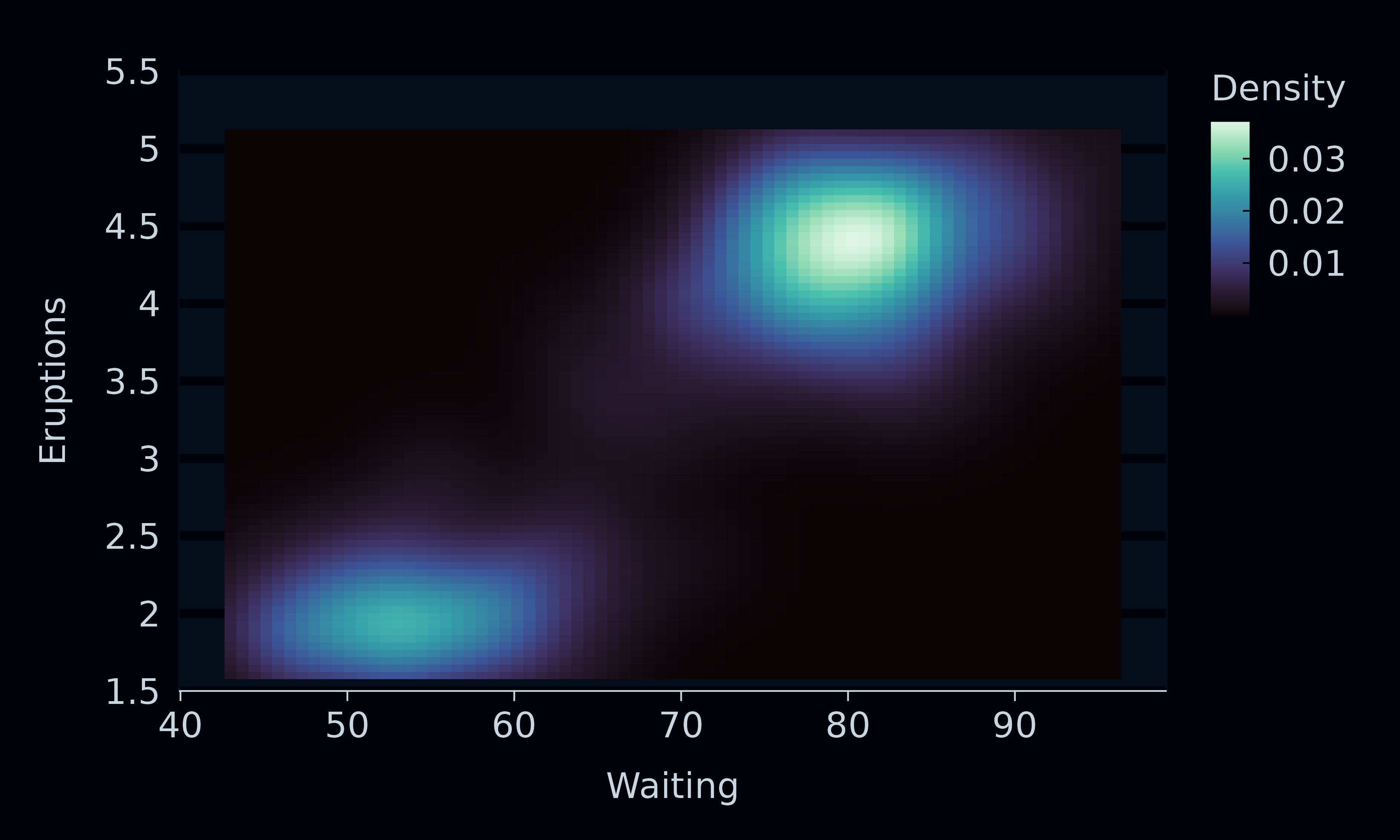
faithful |>
  gg_density_2d_filled(
    x = waiting,
    y = eruptions,
    bins = 8,
    contour = TRUE,
  )

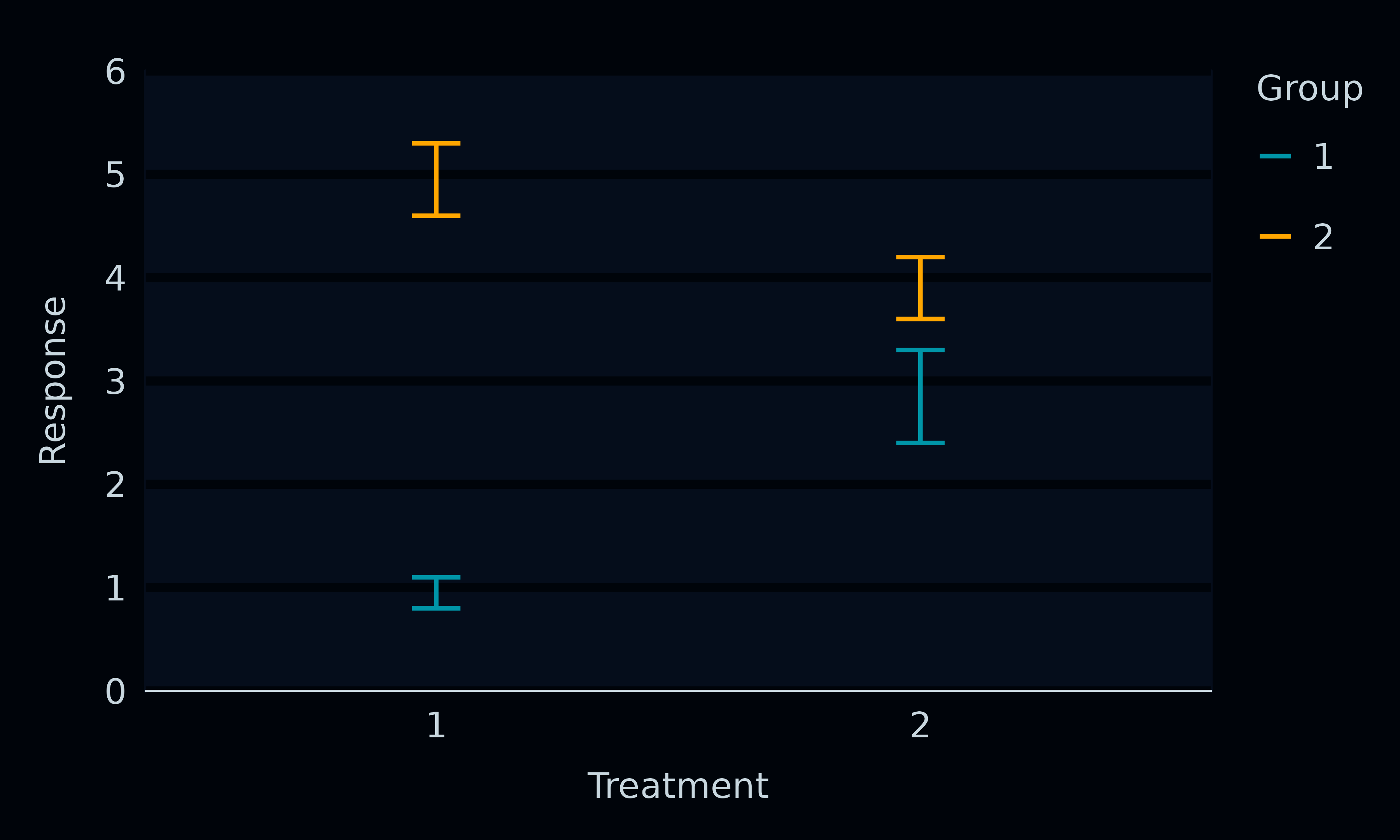
gg_errorbar

experiment |>
  gg_errorbar(
    x = trt,
    ymin = lower,
    ymax = upper,
    col = group,
    y_label = "Response",
    width = 0.1,
    y_expand_limits = 0,
 )

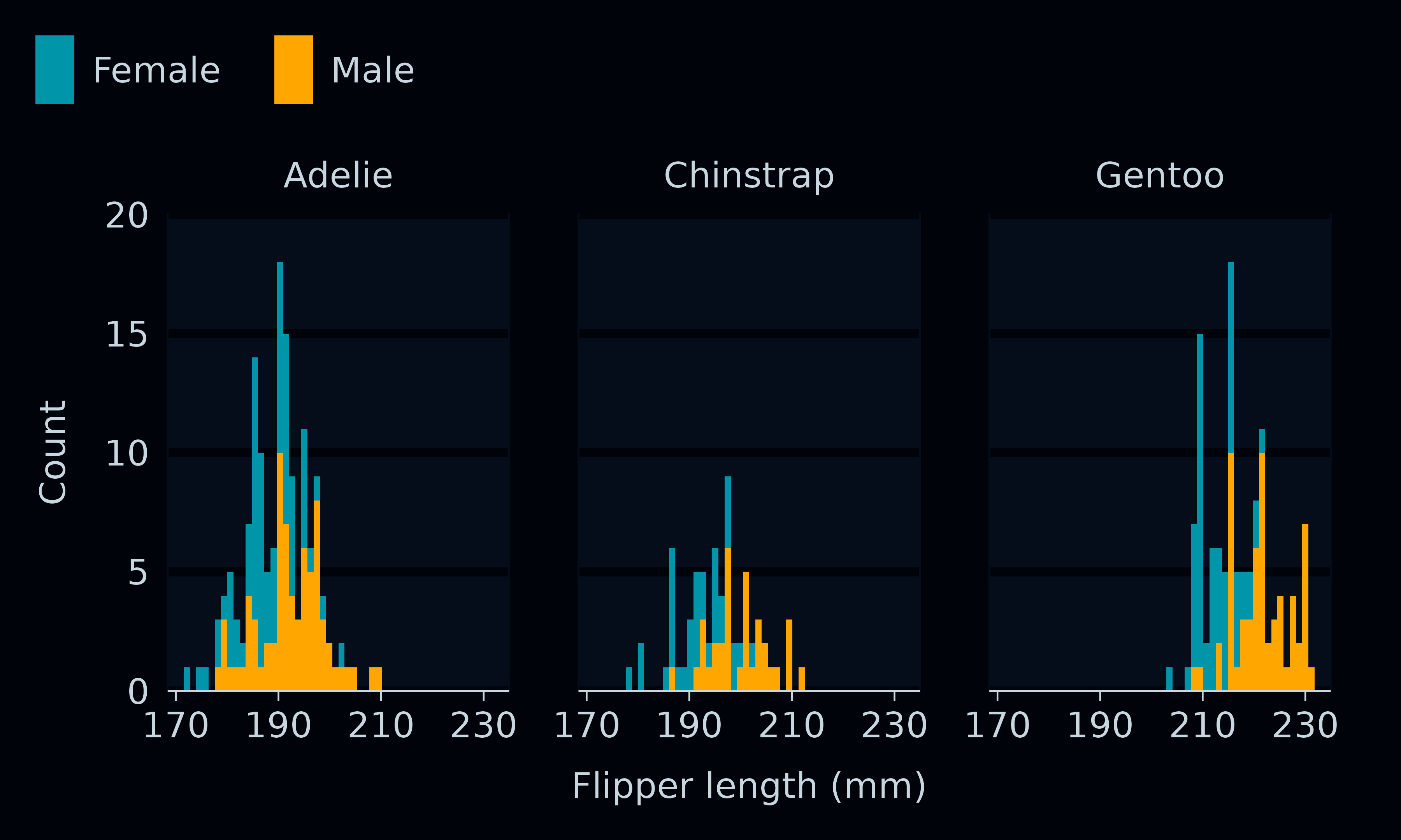
gg_freqpoly

penguins2 |>
  gg_freqpoly(
    x = flipper_length_mm,
    col = sex,
    mode = dark_mode_t(),
  ) +
  theme(legend.title = element_blank())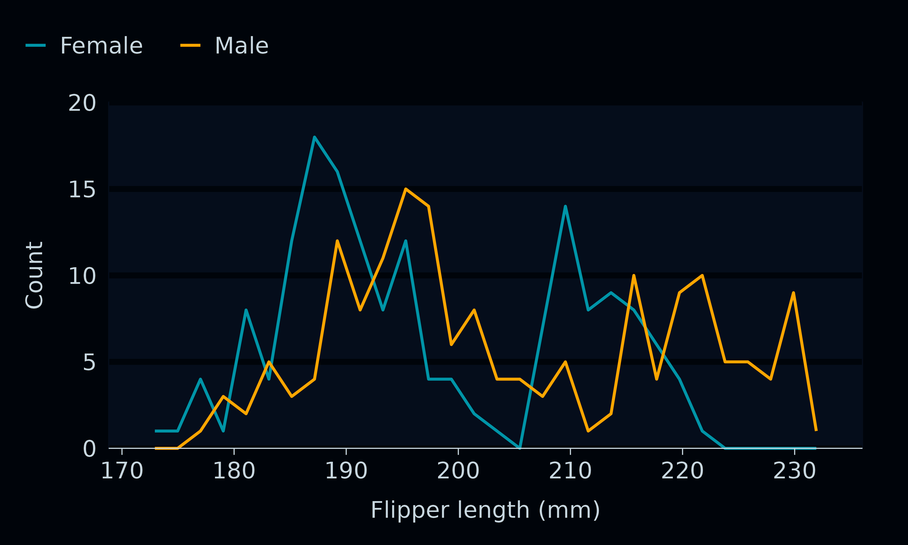

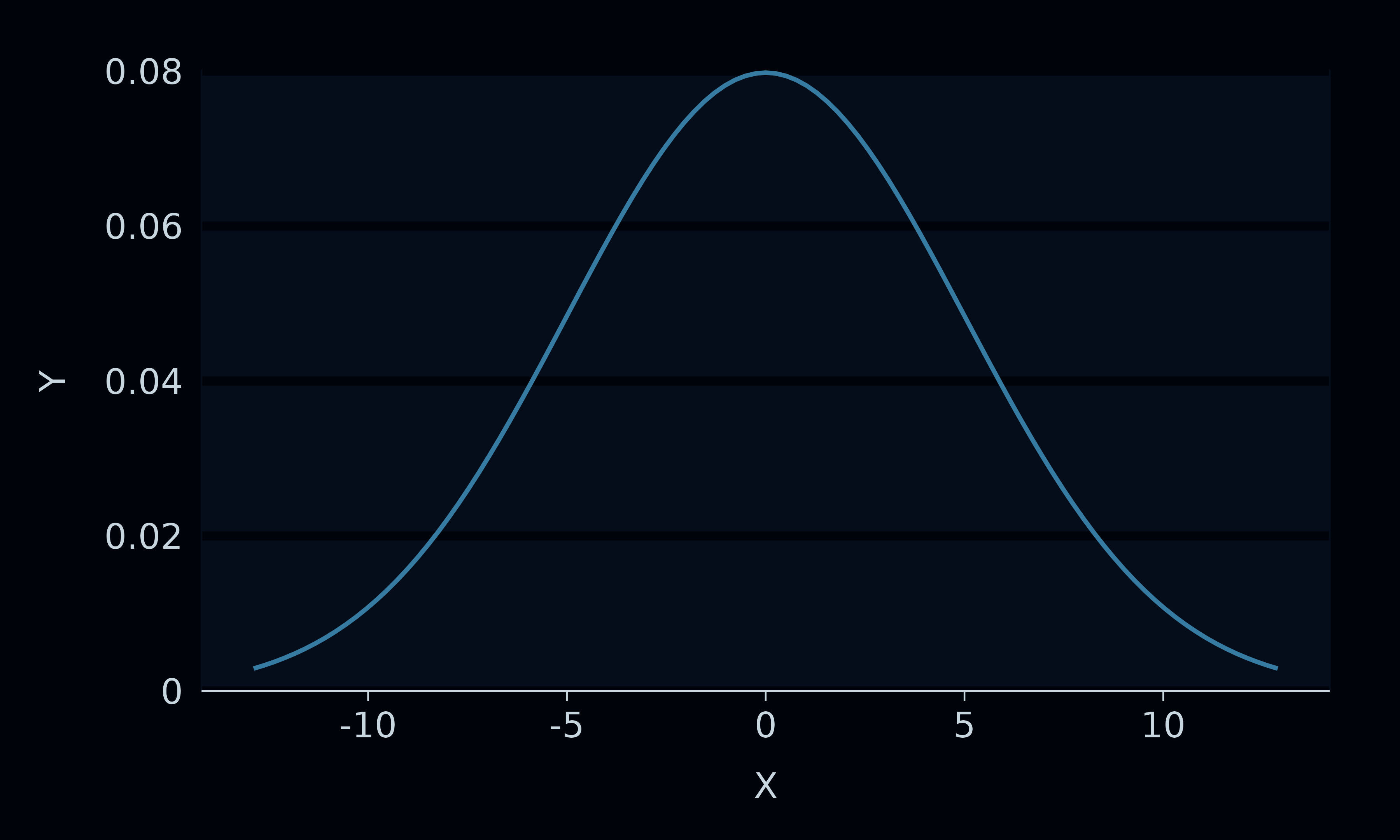
gg_function

gg_function(
  fun = \(x) dnorm(x, mean = 0, sd = 5),
  x_expand_limits = qnorm(p = c(0.005, 0.995), mean = 0, sd = 5),
  x_label = "X",
  y_expand_limits = 0,
)

gg_hex

diamonds |>
  gg_hex(
    x = carat,
    y = price,
  )

gg_histogram

penguins2 |>
  gg_histogram(
    x = flipper_length_mm,
    col = sex,
    facet = species,
    bins = 50,
    mode = dark_mode_t(),
  ) +
  theme(legend.title = element_blank())

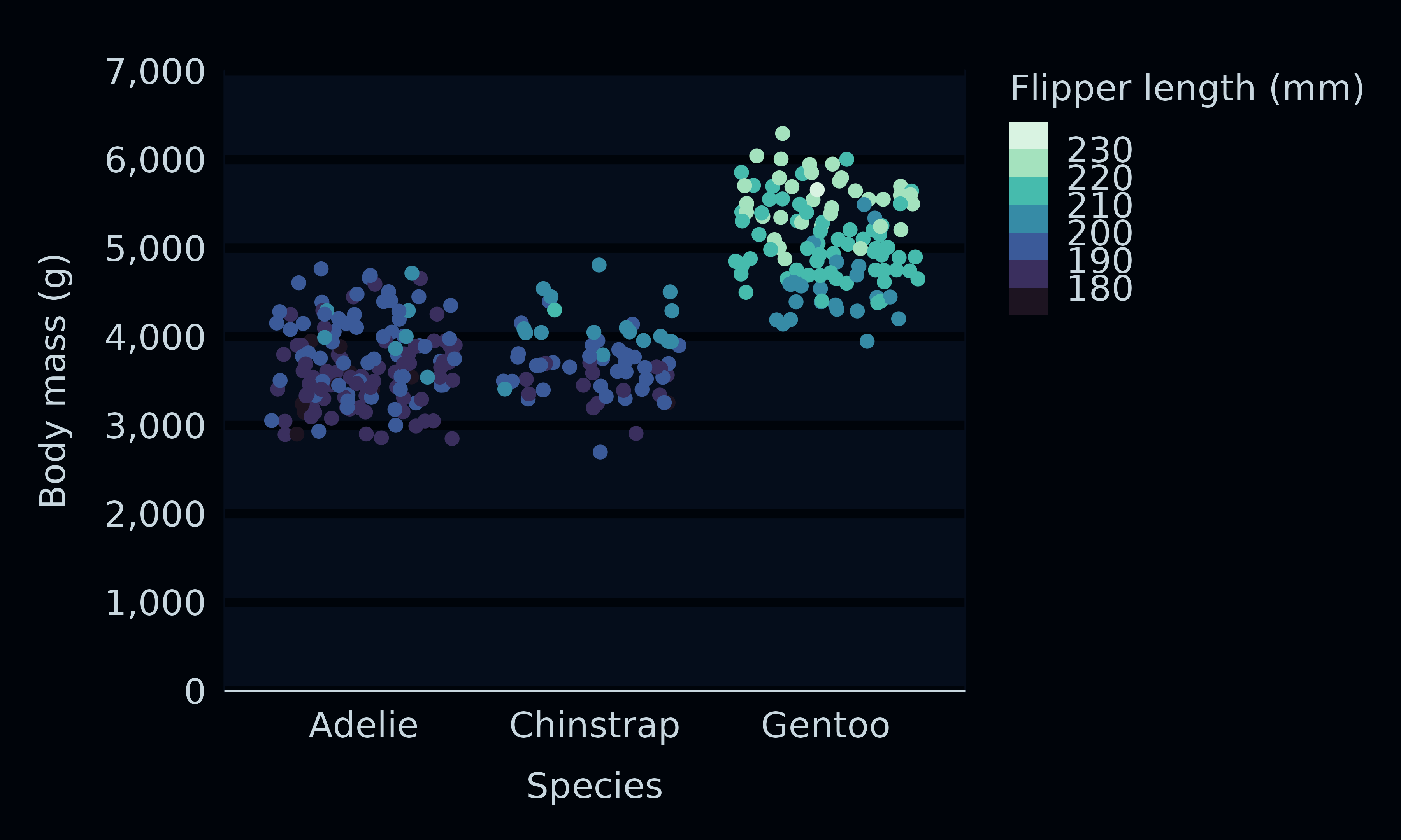
gg_jitter

set.seed(123)

penguins2 |>
  gg_jitter(
    position = position_jitter(), 
    x = species,
    y = body_mass_g,
    col = flipper_length_mm,
    y_expand_limits = 0,
    col_steps = TRUE,
  )

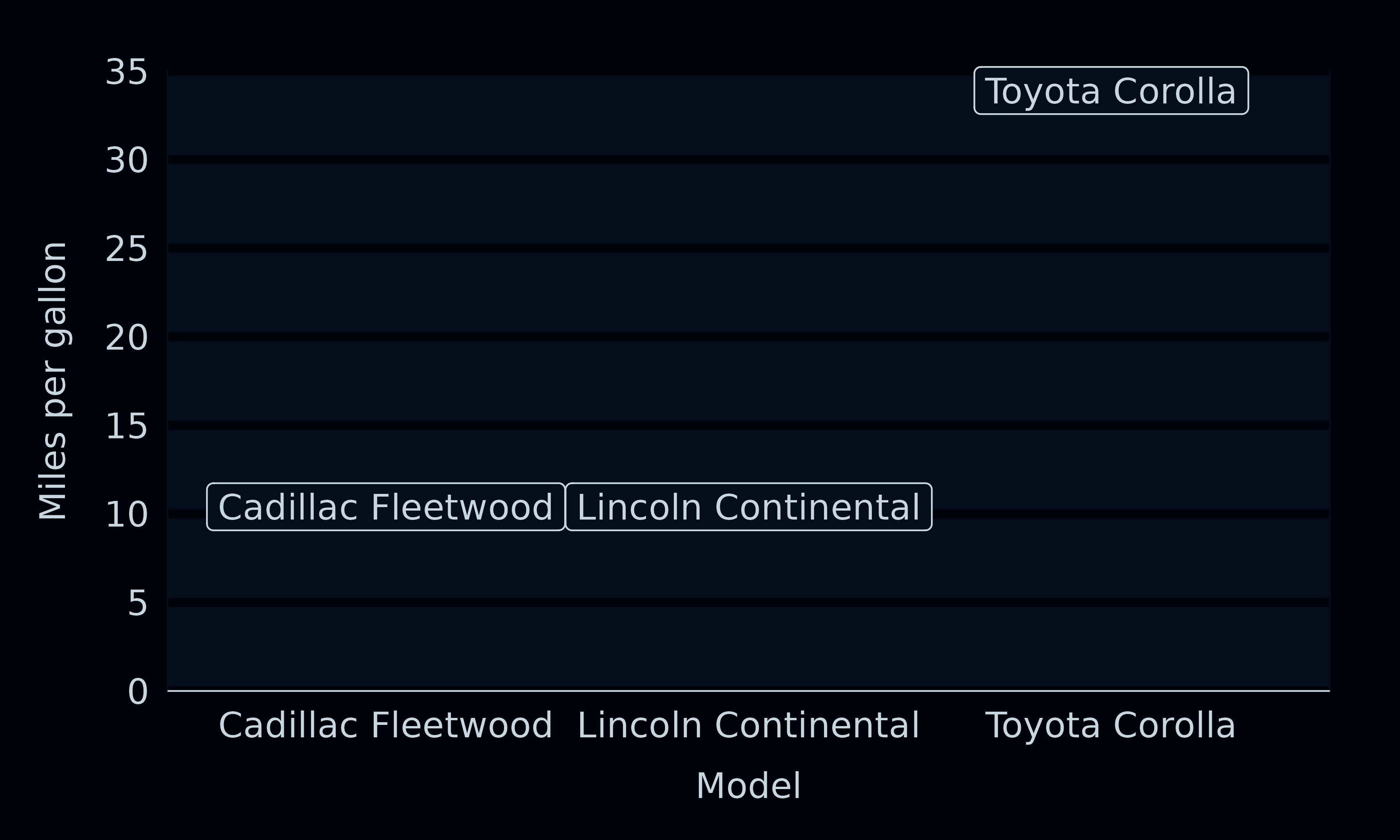
gg_label

bind_rows(
  mtcars |> slice_min(order_by = mpg),
  mtcars |> slice_max(order_by = mpg)) |>
  tibble::rownames_to_column("model") |>
  gg_label(
    x = model,
    y = mpg,
    label = model,
    fill = darkness[3],
    y_expand_limits = 0,
    y_label = "Miles per gallon", 
  )

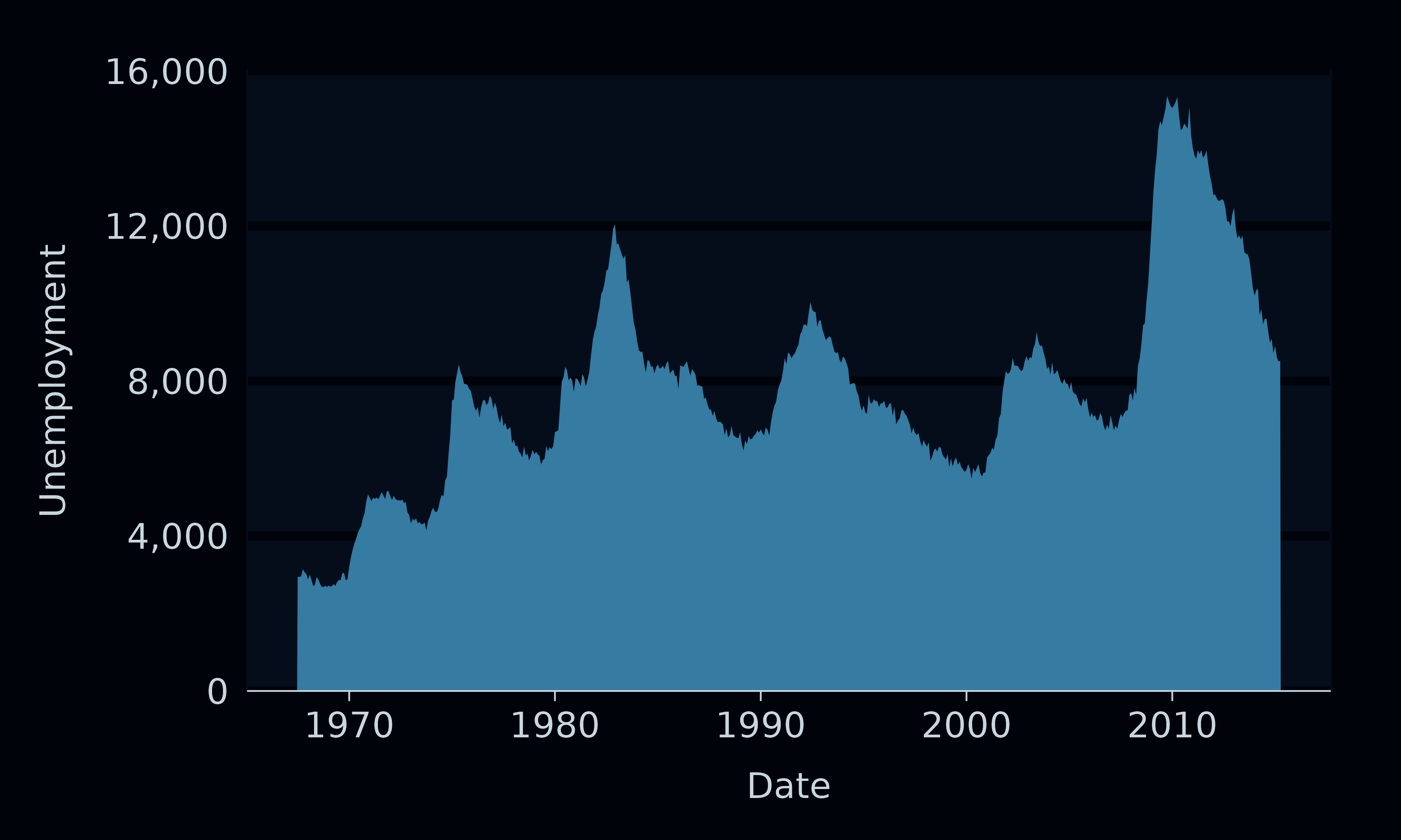
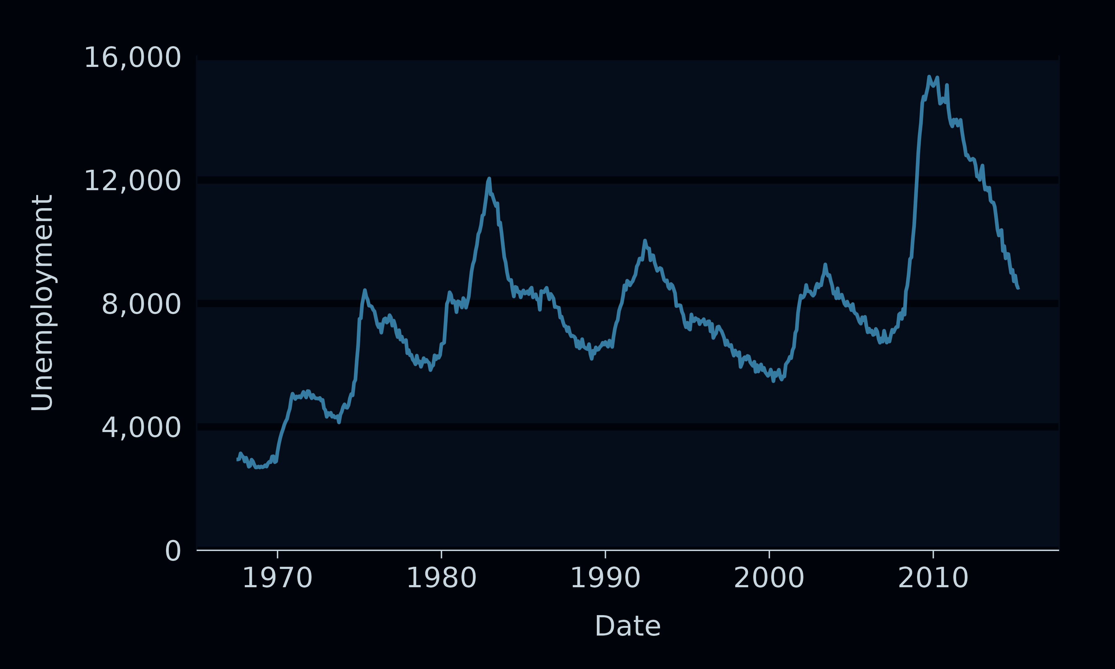
gg_line

economics |>
  gg_line(
    x = date,
    y = unemploy,
    y_expand_limits = 0, 
    y_label = "Unemployment",
  )

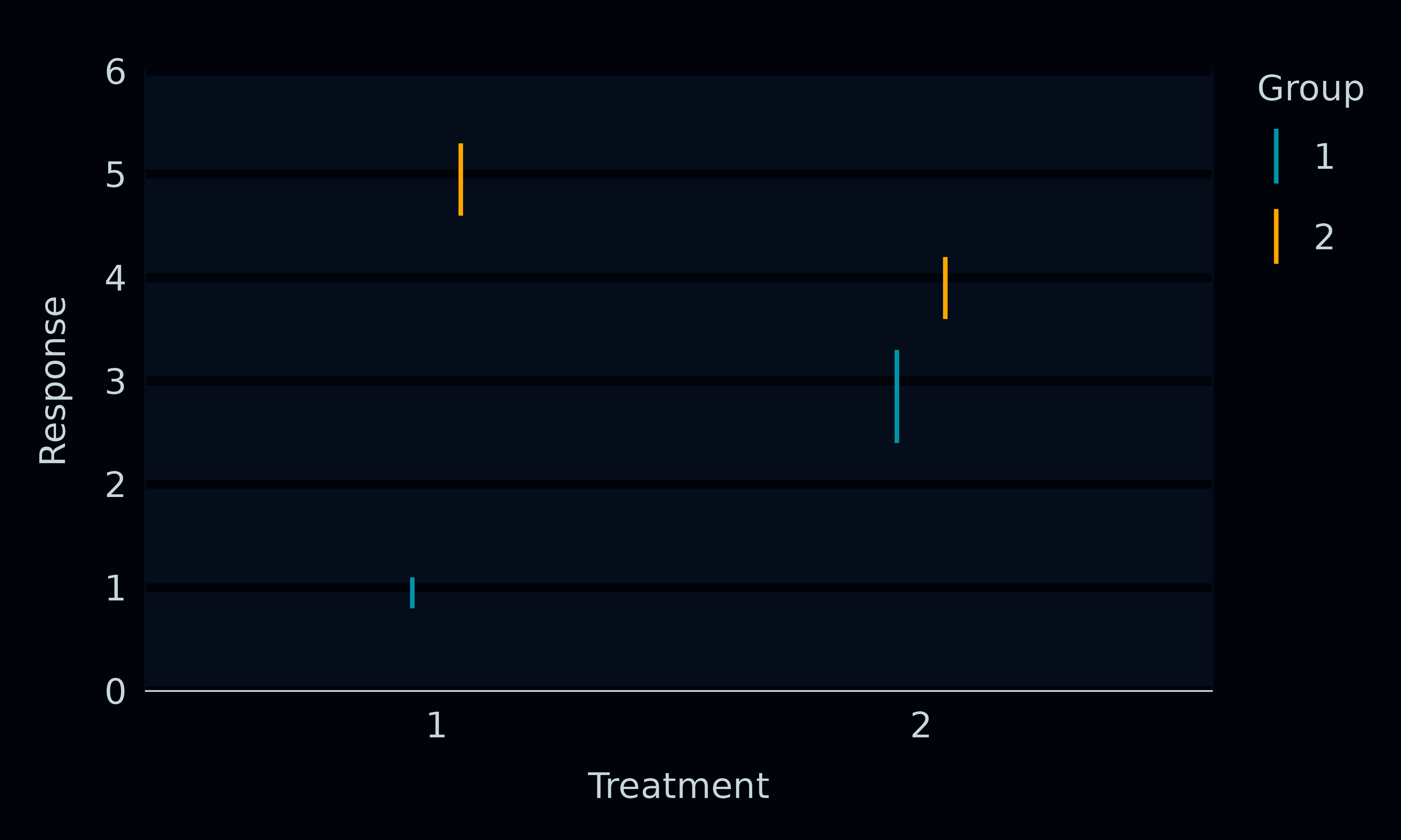
gg_linerange

experiment |>
  gg_linerange(
    position = position_dodge(width = 0.2),
    x = trt,
    ymin = lower,
    ymax = upper,
    col = group,
    y_label = "Response",
    y_expand_limits = 0,
  )

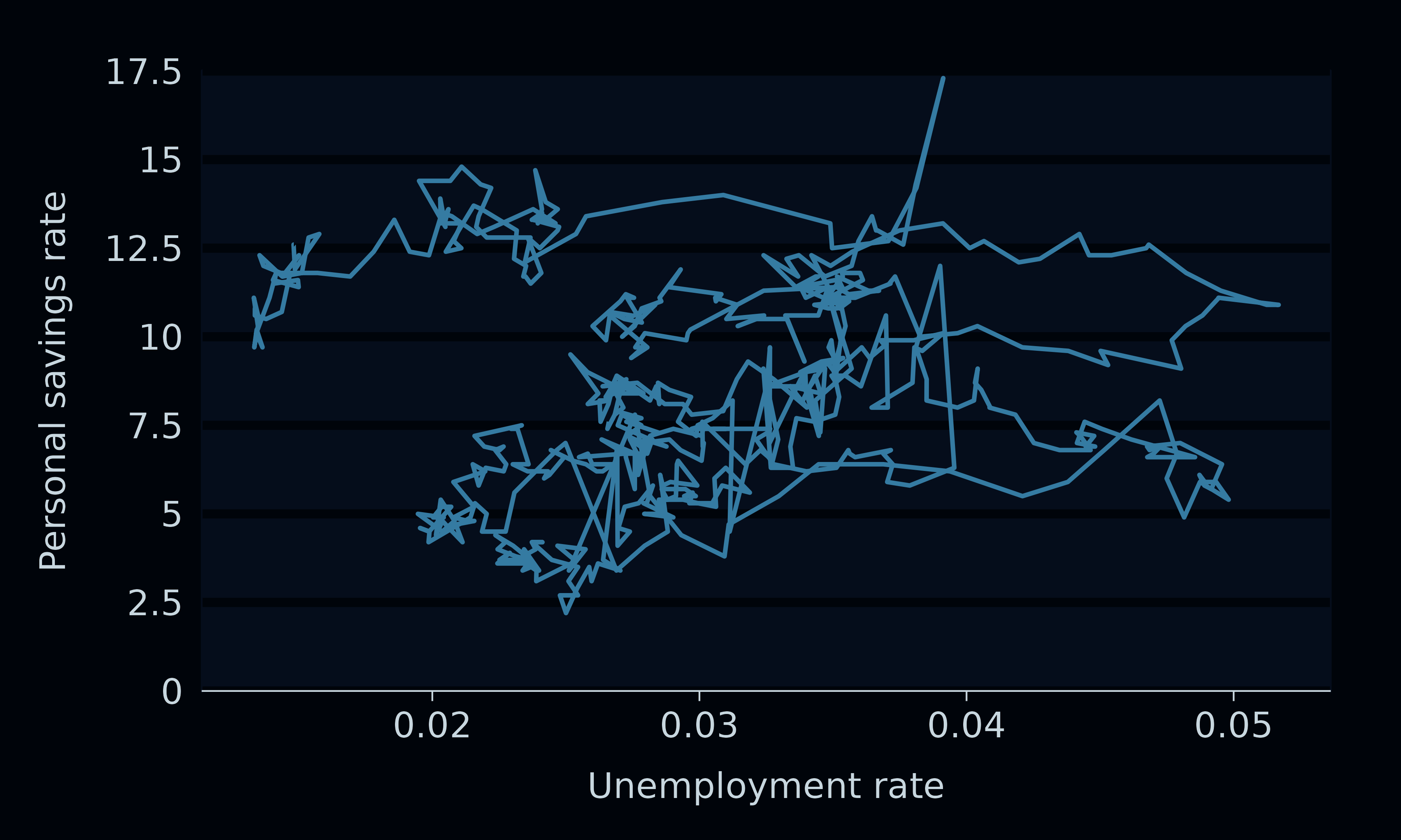
gg_path

economics |>
  mutate(unemploy_rate = unemploy / pop) |>
  gg_path(
    x = unemploy_rate,
    y = psavert,
    x_label = "Unemployment rate",
    y_expand_limits = 0,
    y_label = "Personal savings rate",
  )

gg_point

penguins2 |>
  gg_point(
    x = flipper_length_mm,
    y = body_mass_g, 
    col = species,
  )

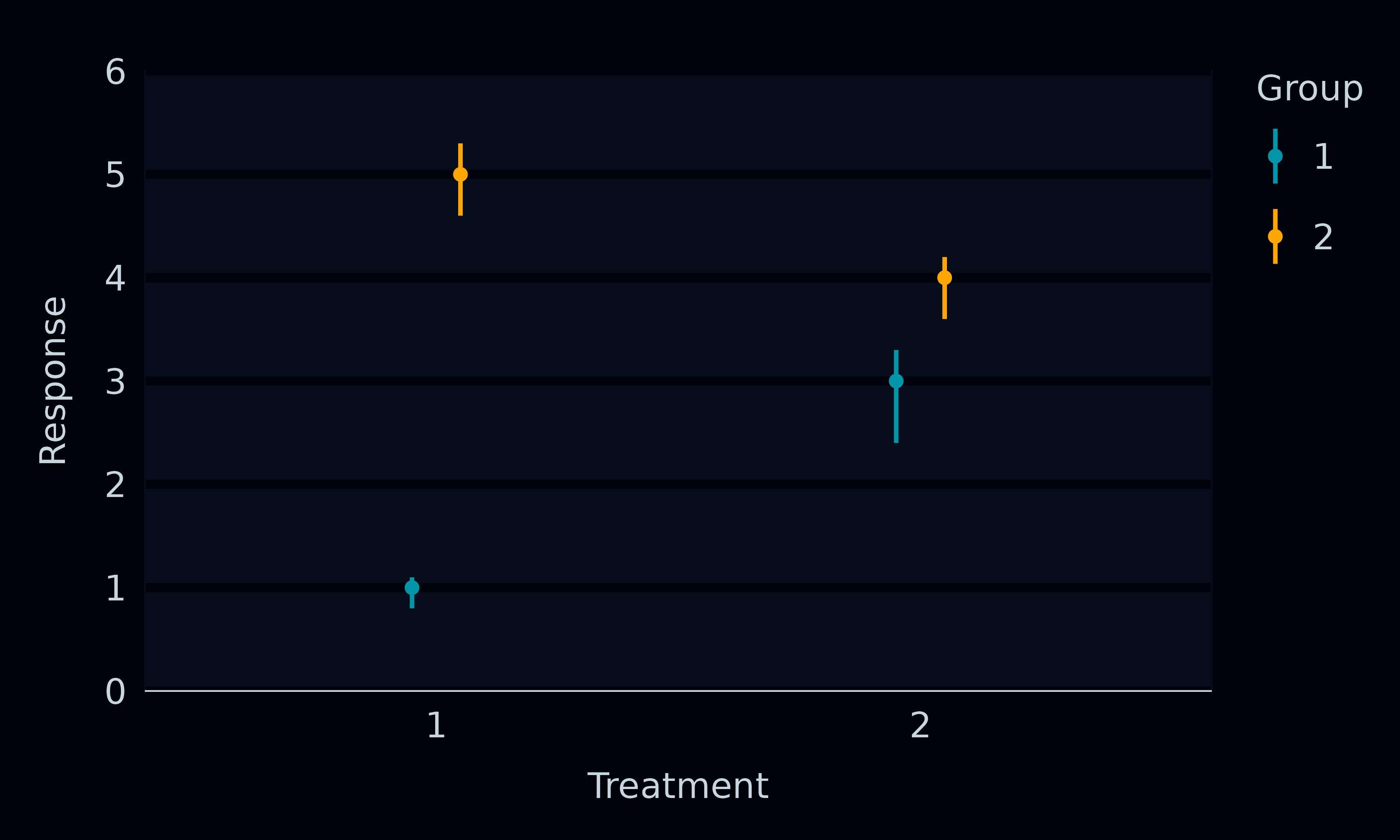
gg_pointrange

experiment |>
  gg_pointrange(
    position = position_dodge(width = 0.2),
    x = trt,
    y = resp,
    col = group,
    ymin = lower,
    ymax = upper,
    y_expand_limits = 0,
  )

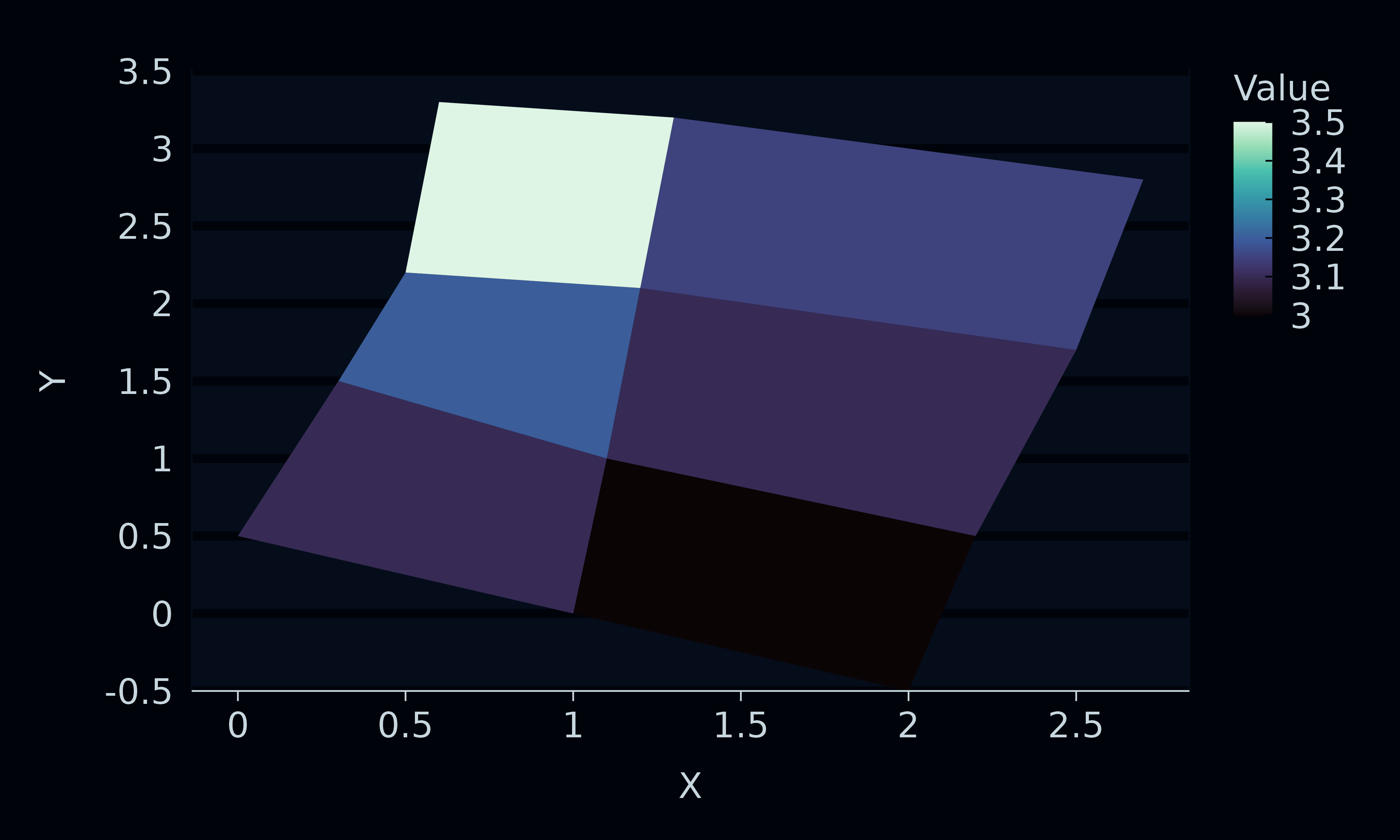
gg_polygon

ids <- factor(c("1.1", "2.1", "1.2", "2.2", "1.3", "2.3"))

values <- data.frame(
  id = ids,
  value = c(3, 3.1, 3.1, 3.2, 3.15, 3.5)
)

positions <- data.frame(
  id = rep(ids, each = 4),
  x = c(2, 1, 1.1, 2.2, 1, 0, 0.3, 1.1, 2.2, 1.1, 1.2, 2.5, 1.1, 0.3,
        0.5, 1.2, 2.5, 1.2, 1.3, 2.7, 1.2, 0.5, 0.6, 1.3),
  y = c(-0.5, 0, 1, 0.5, 0, 0.5, 1.5, 1, 0.5, 1, 2.1, 1.7, 1, 1.5,
        2.2, 2.1, 1.7, 2.1, 3.2, 2.8, 2.1, 2.2, 3.3, 3.2)
)

datapoly <- merge(values, positions, by = c("id"))

datapoly |>
  gg_polygon(
    x = x,
    y = y,
    col = value,
    group = id, 
  )

gg_qq

penguins2 |>
  gg_qq(
    sample = body_mass_g,
    facet = species,
    coord = coord_cartesian(clip = "on"), 
  ) +
  geom_qq_line()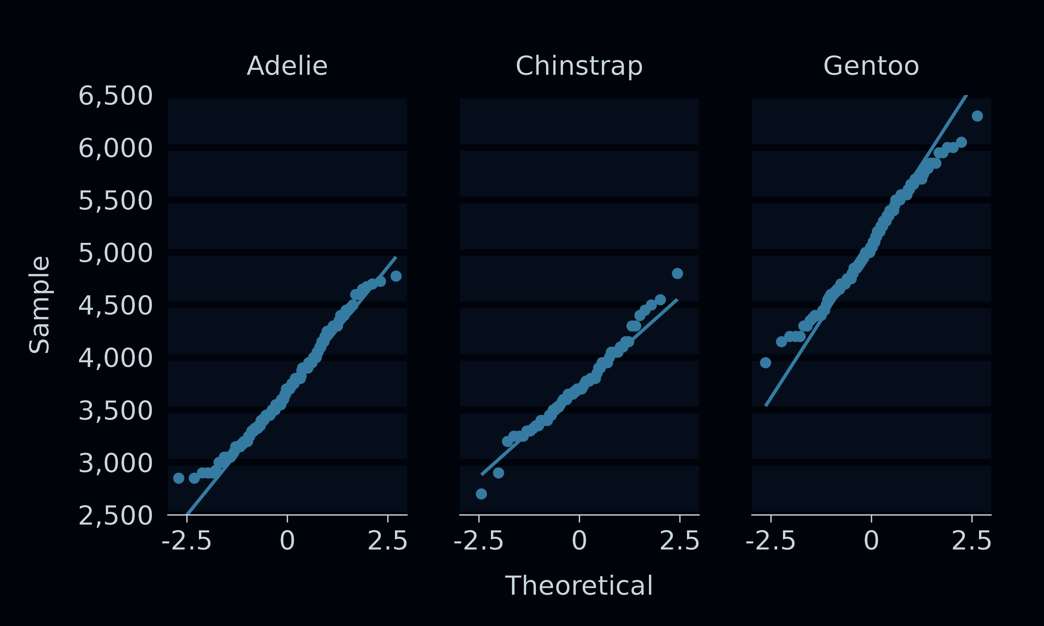

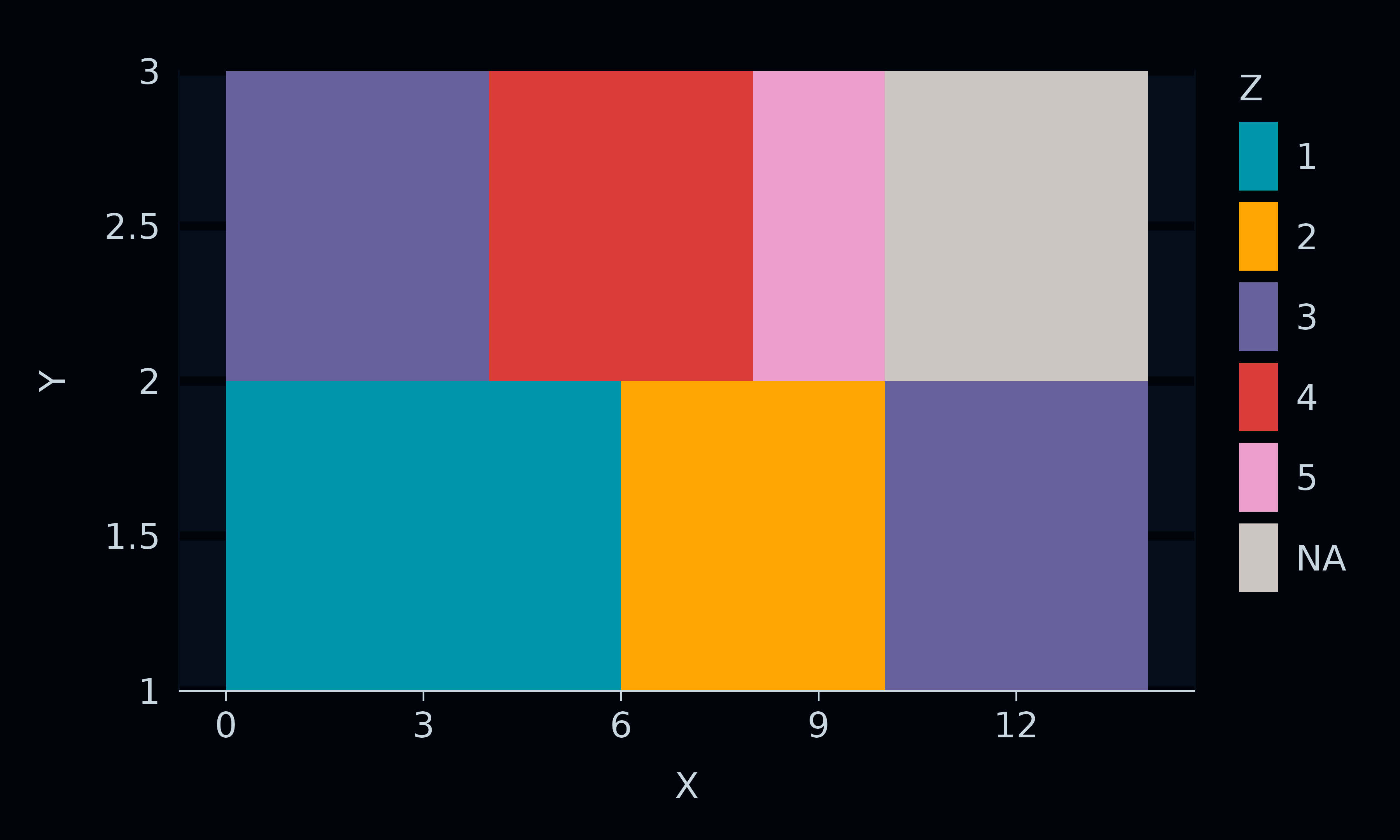
gg_quantile

penguins2 |>
  gg_quantile(
    x = flipper_length_mm,
    y = body_mass_g,
  )

gg_raster

faithfuld |>
  gg_raster(
    x = waiting,
    y = eruptions,
    col = density,
  )

gg_rect

data.frame(
  x = rep(c(2, 5, 7, 9, 12), 2),
  y = rep(c(1, 2), each = 5),
  z = factor(c(rep(1:4, each = 2), 5, NA)),
  w = rep(diff(c(0, 4, 6, 8, 10, 14)), 2)) |>
  mutate(
    xmin = x - w / 2,
    xmax = x + w / 2,
    ymin = y,
    ymax = y + 1
  ) |>
  gg_rect(
    xmin = xmin,
    xmax = xmax,
    ymin = ymin,
    ymax = ymax,
    col = z,
  )

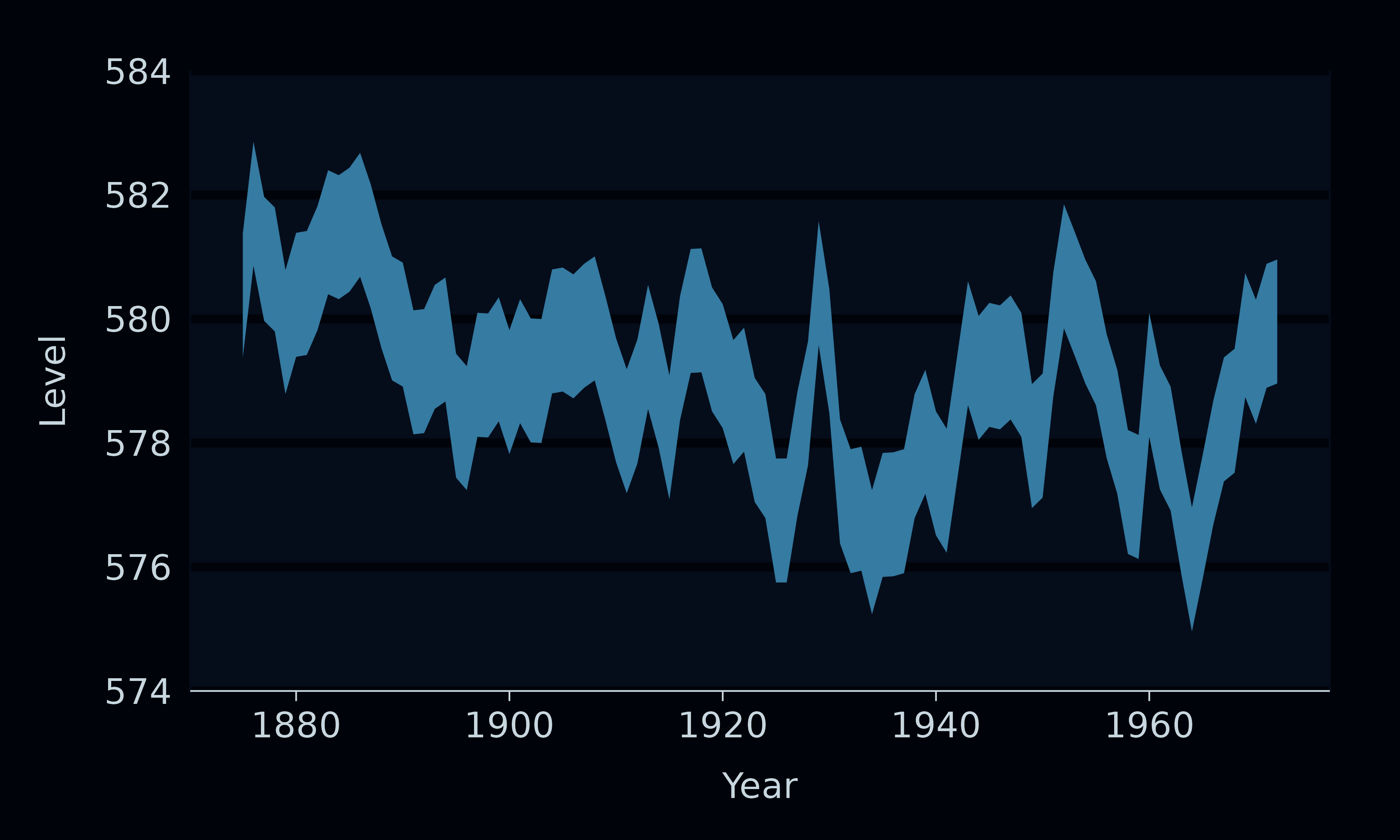
gg_ribbon

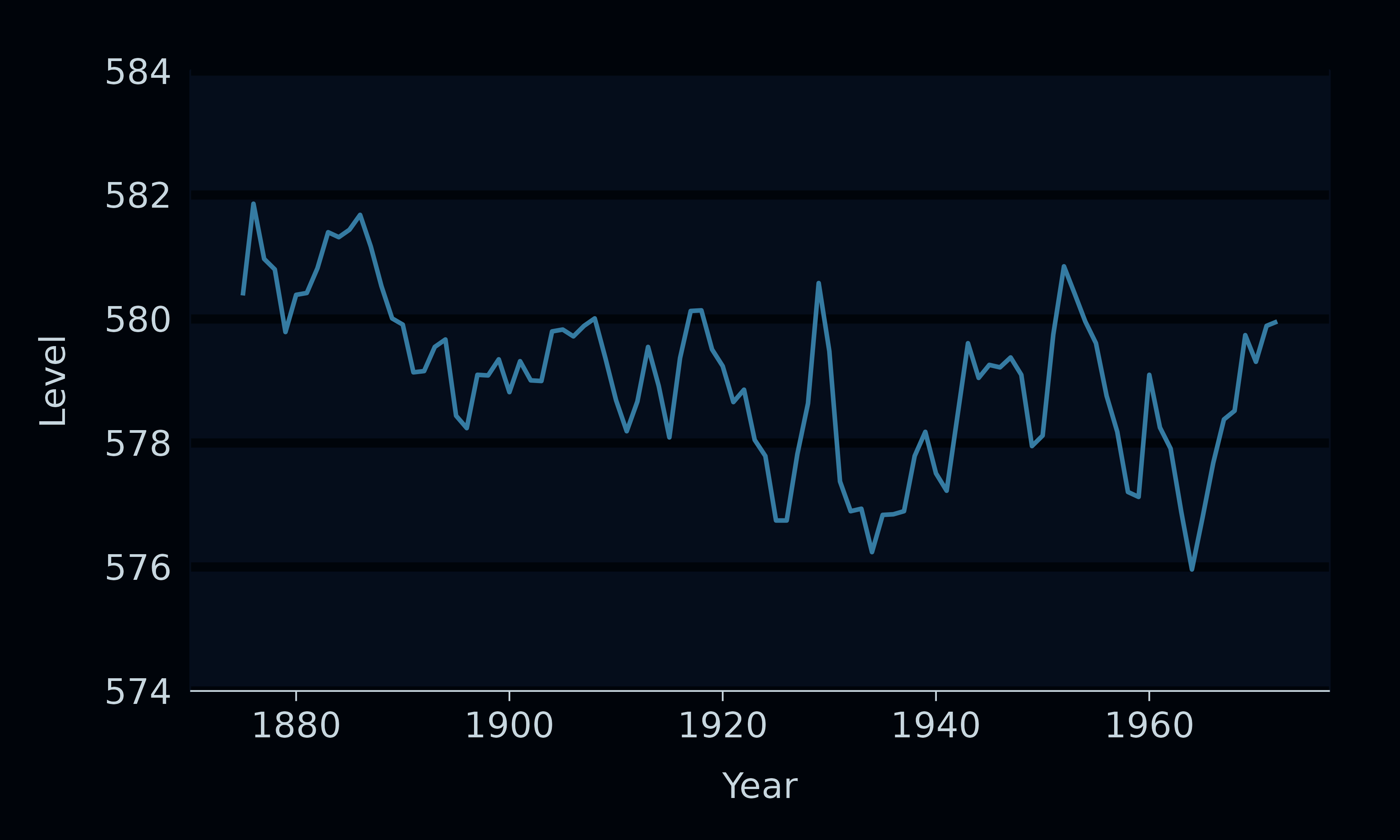
data.frame(year = 1875:1972, level = as.vector(LakeHuron)) |>
  mutate(level_min = level - 1, level_max = level + 1) |>
  gg_ribbon(
    x = year,
    ymin = level_min,
    ymax = level_max,
    x_labels = \(x) x,
    y_label = "Level",
  ) 

gg_ribbon_line

data.frame(year = 1875:1972, level = as.vector(LakeHuron)) |>
  mutate(level_min = level - 1, level_max = level + 1) |>
  gg_ribbon_line(
    x = year,
    y = level,
    ymin = level_min,
    ymax = level_max,
    x_labels = \(x) x,
    blend = "multiply",
  )

gg_rug

penguins2 |>
  gg_rug(
    x = flipper_length_mm,
    y = body_mass_g,
    col = sex,
  )

gg_segment

data.frame(x1 = 2.62, x2 = 3.57, y1 = 21.0, y2 = 15.0) |>
  gg_segment(
    x = x1,
    xend = x2,
    y = y1,
    yend = y2,
  )

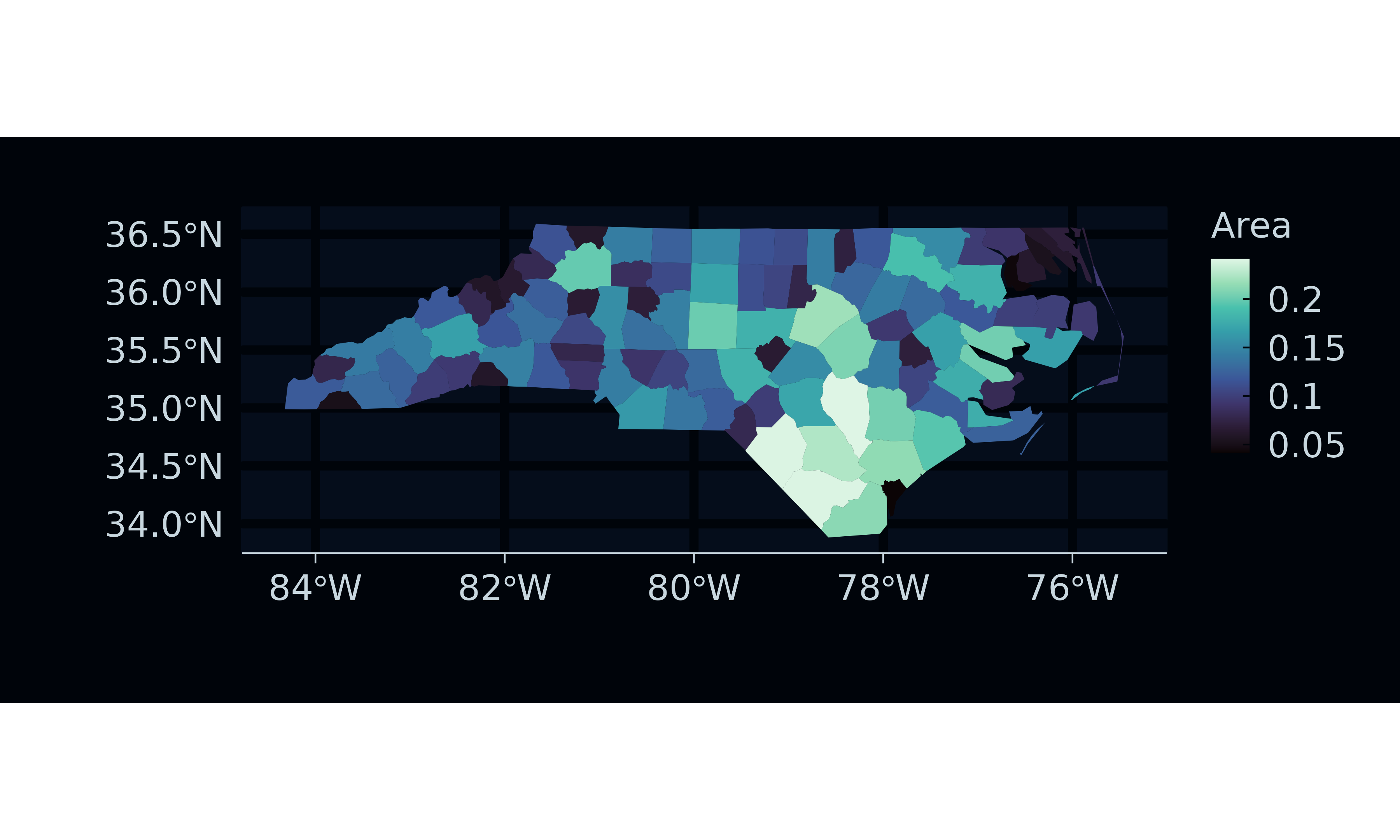
gg_sf

sf::st_read(system.file("shape/nc.shp", package = "sf")) |> 
  gg_sf(
    col = AREA, 
  )
#> Reading layer `nc' from data source 
#>   `/home/runner/work/_temp/Library/sf/shape/nc.shp' using driver `ESRI Shapefile'
#> Simple feature collection with 100 features and 14 fields
#> Geometry type: MULTIPOLYGON
#> Dimension:     XY
#> Bounding box:  xmin: -84.32385 ymin: 33.88199 xmax: -75.45698 ymax: 36.58965
#> Geodetic CRS:  NAD27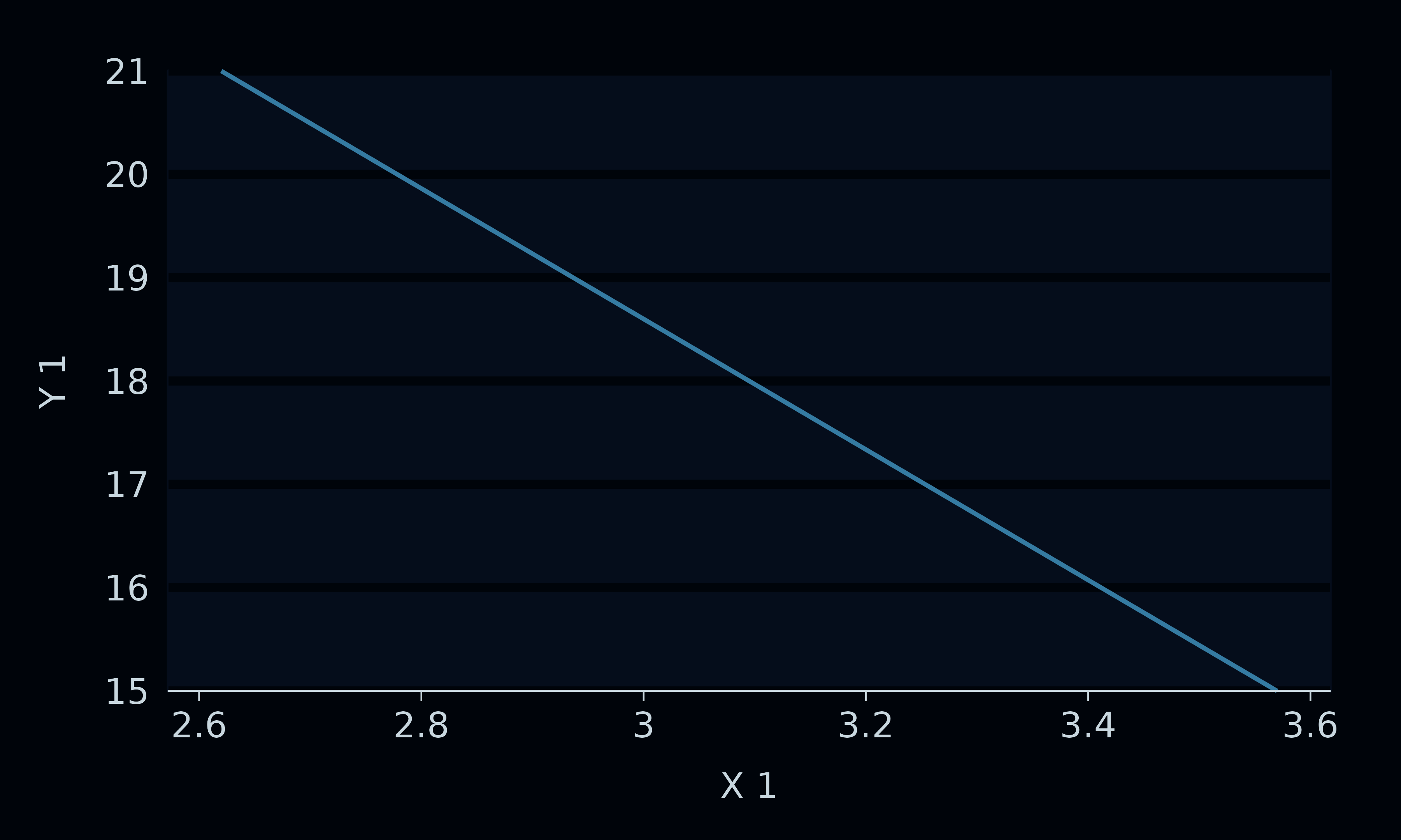

gg_smooth

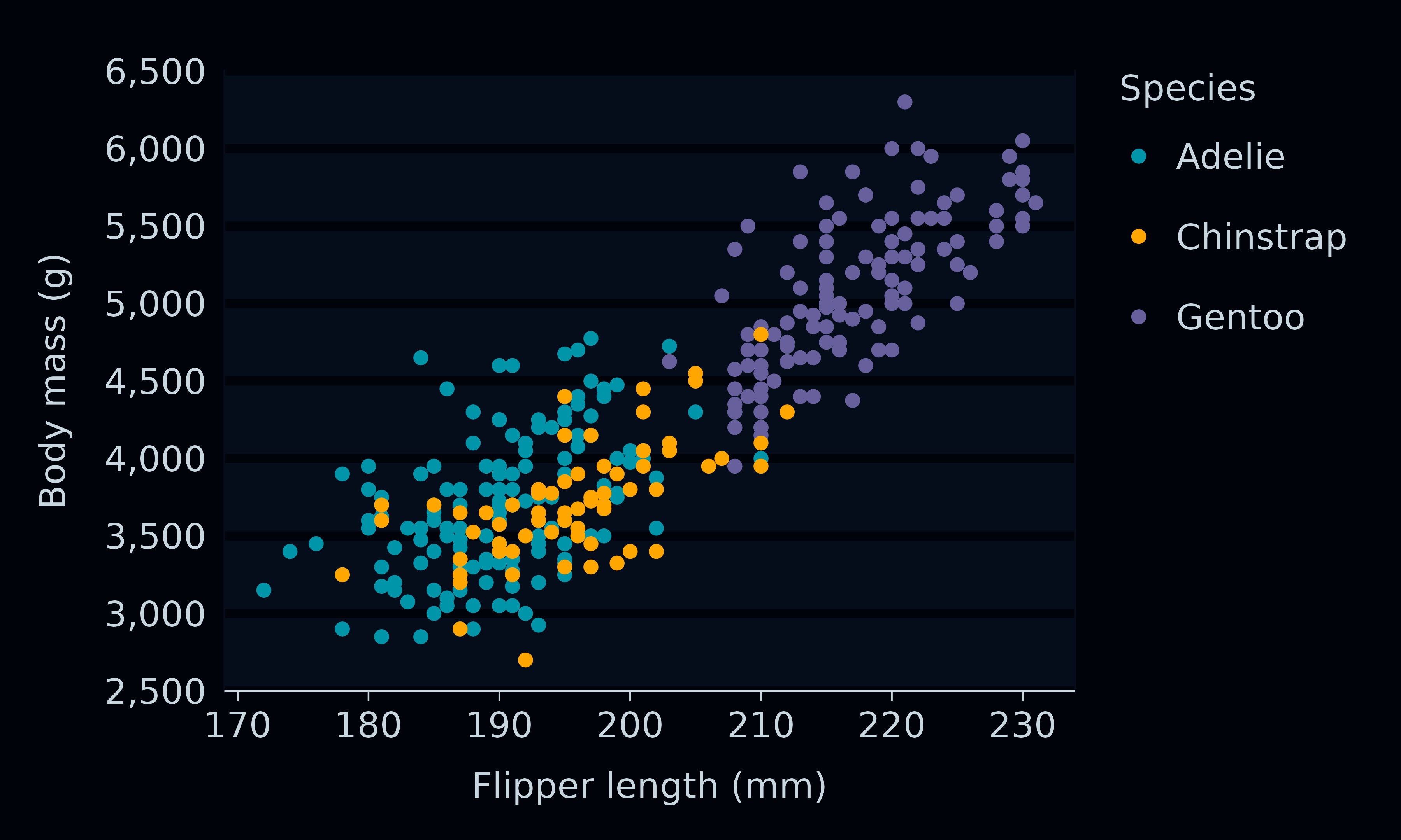
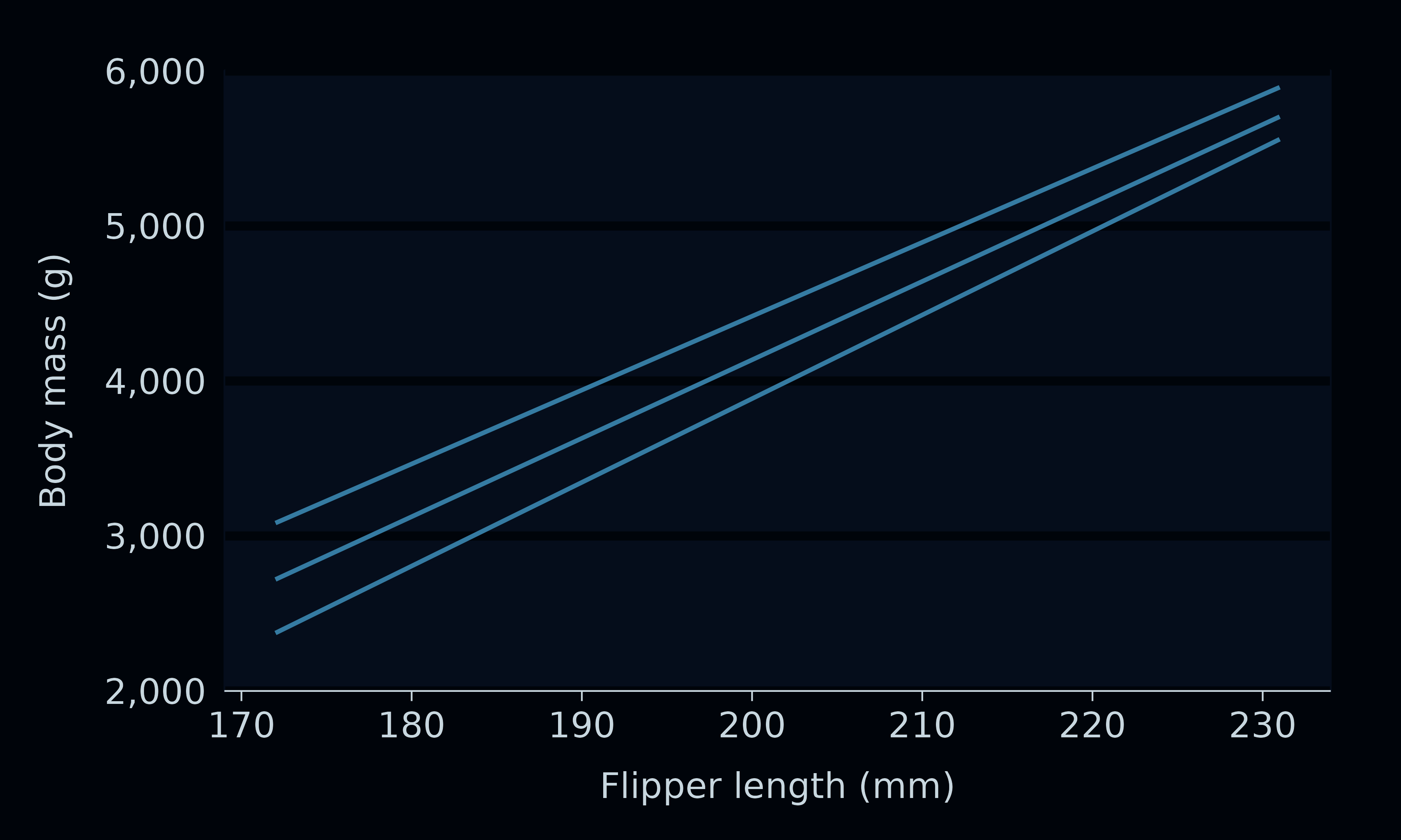
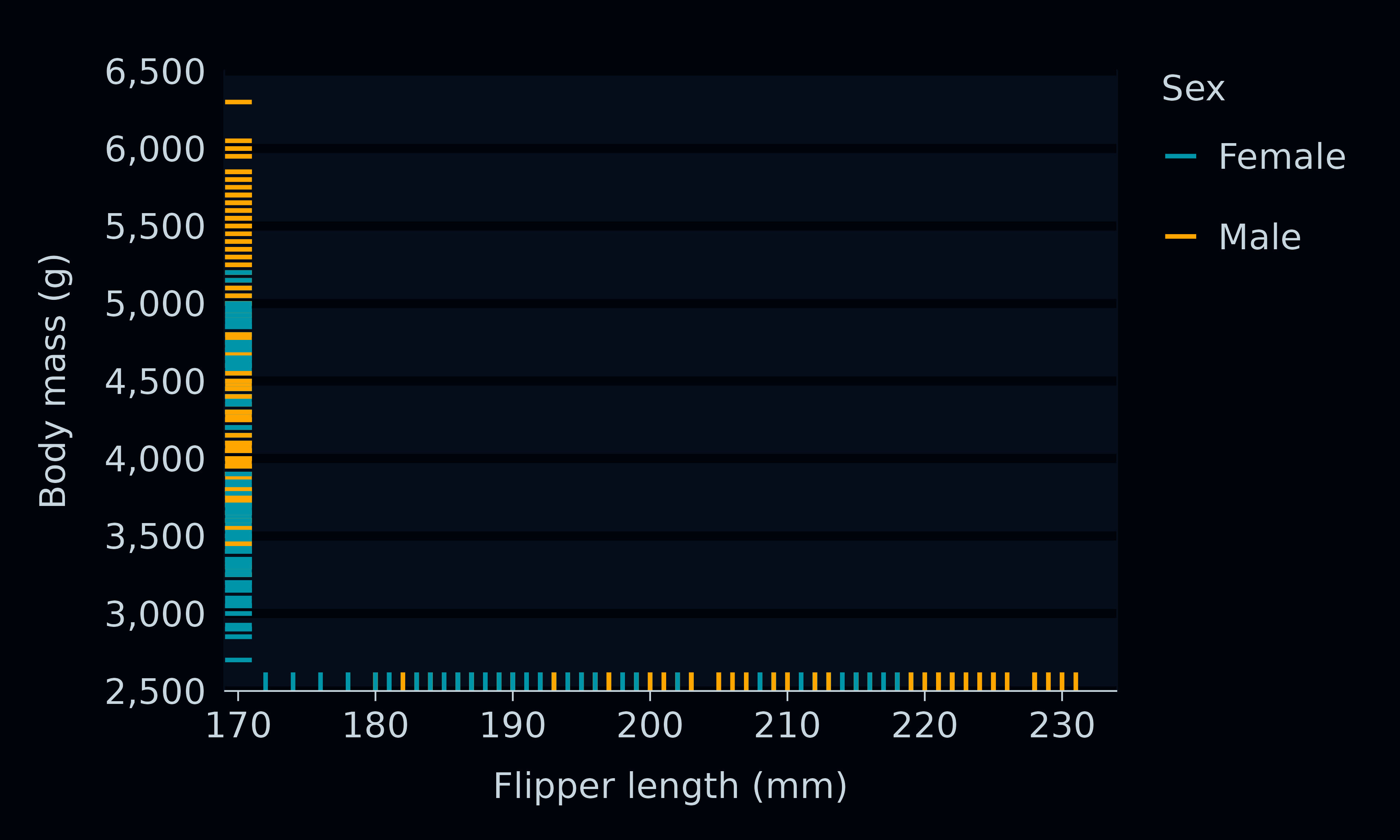
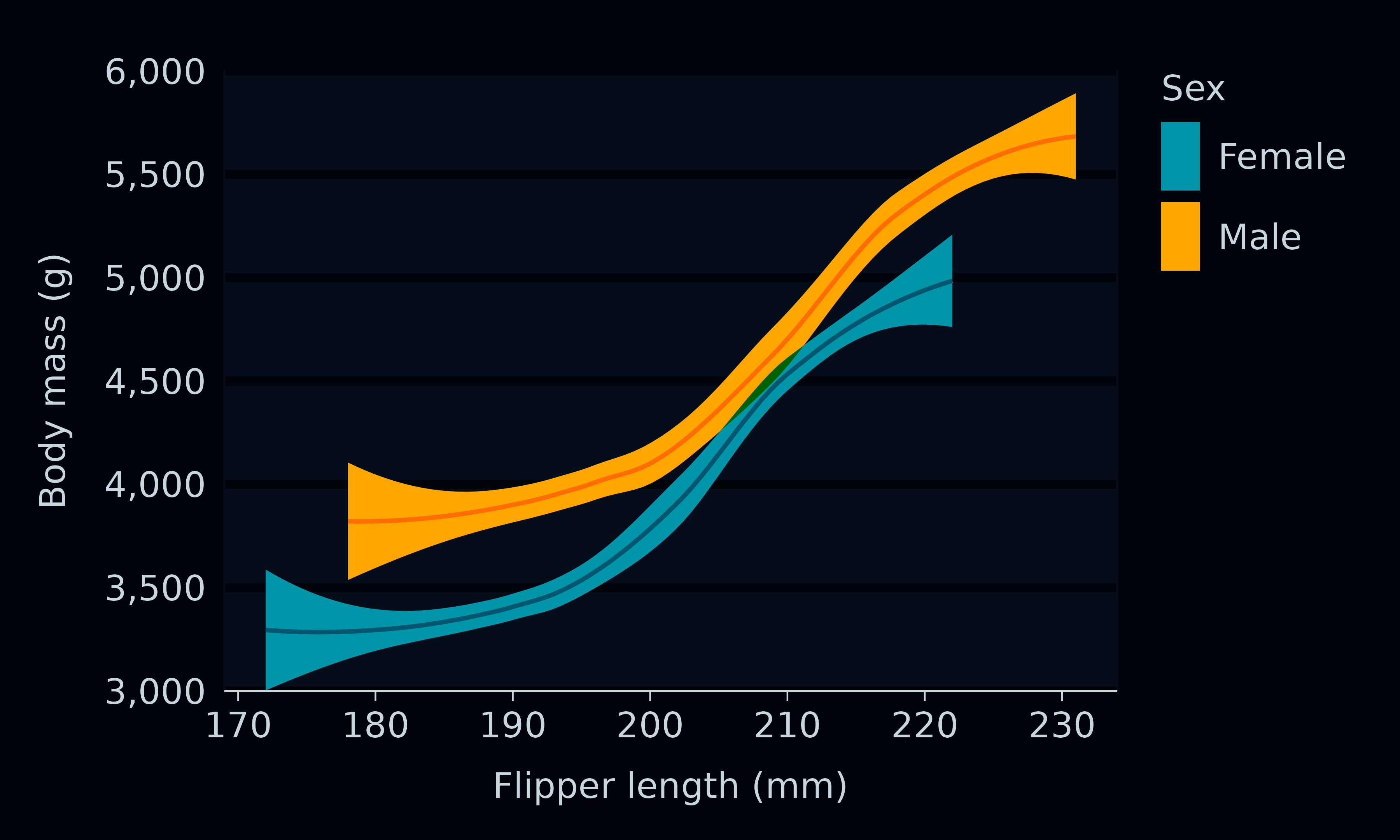
penguins2 |>
  gg_smooth(
    x = flipper_length_mm,
    y = body_mass_g,
    col = sex,
    blend = "multiply",
    se = TRUE,
  )

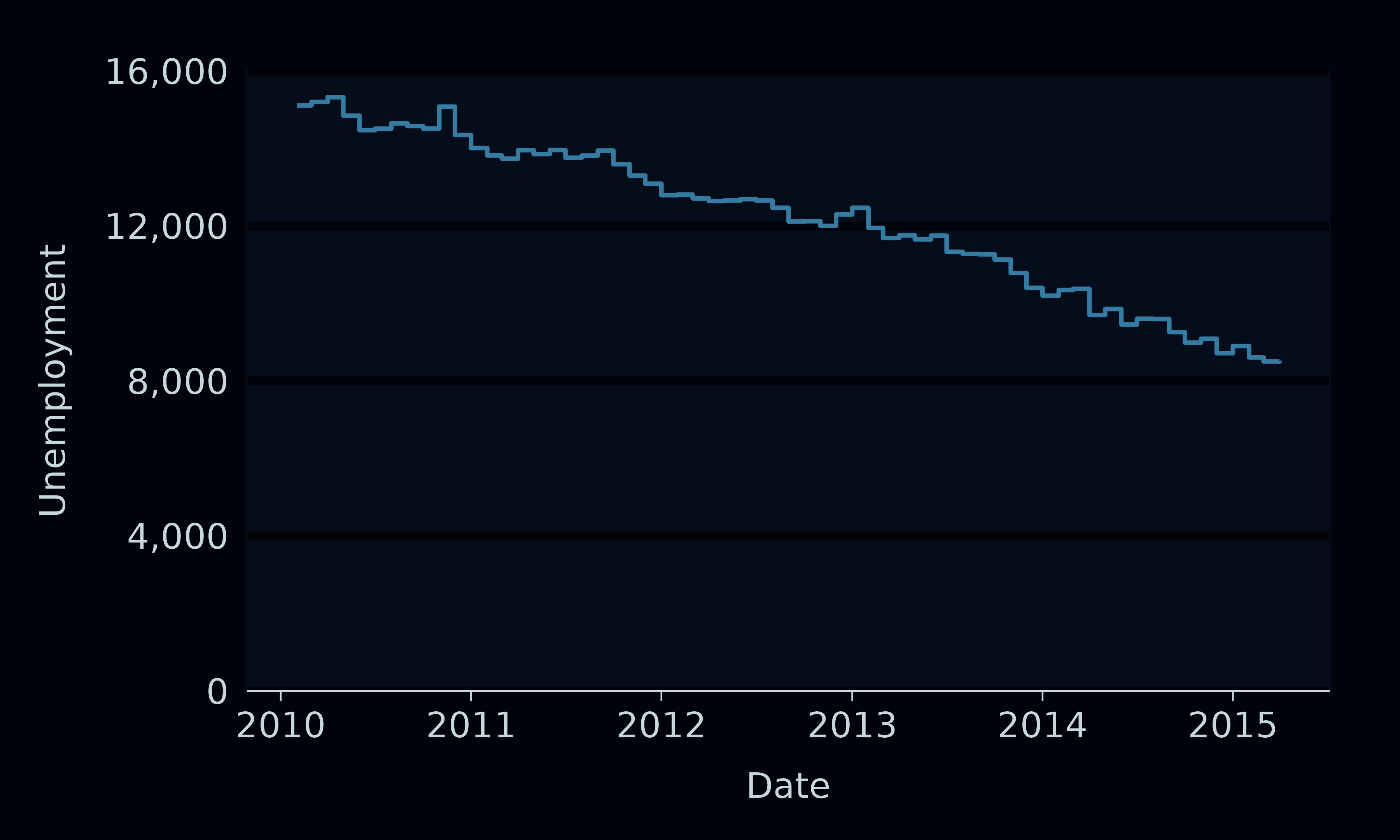
gg_step

economics |>
  filter(date > lubridate::ymd("2010-01-01")) |>  
  gg_step(
    x = date,
    y = unemploy,
    y_expand_limits = 0,
    y_label = "Unemployment",
  )

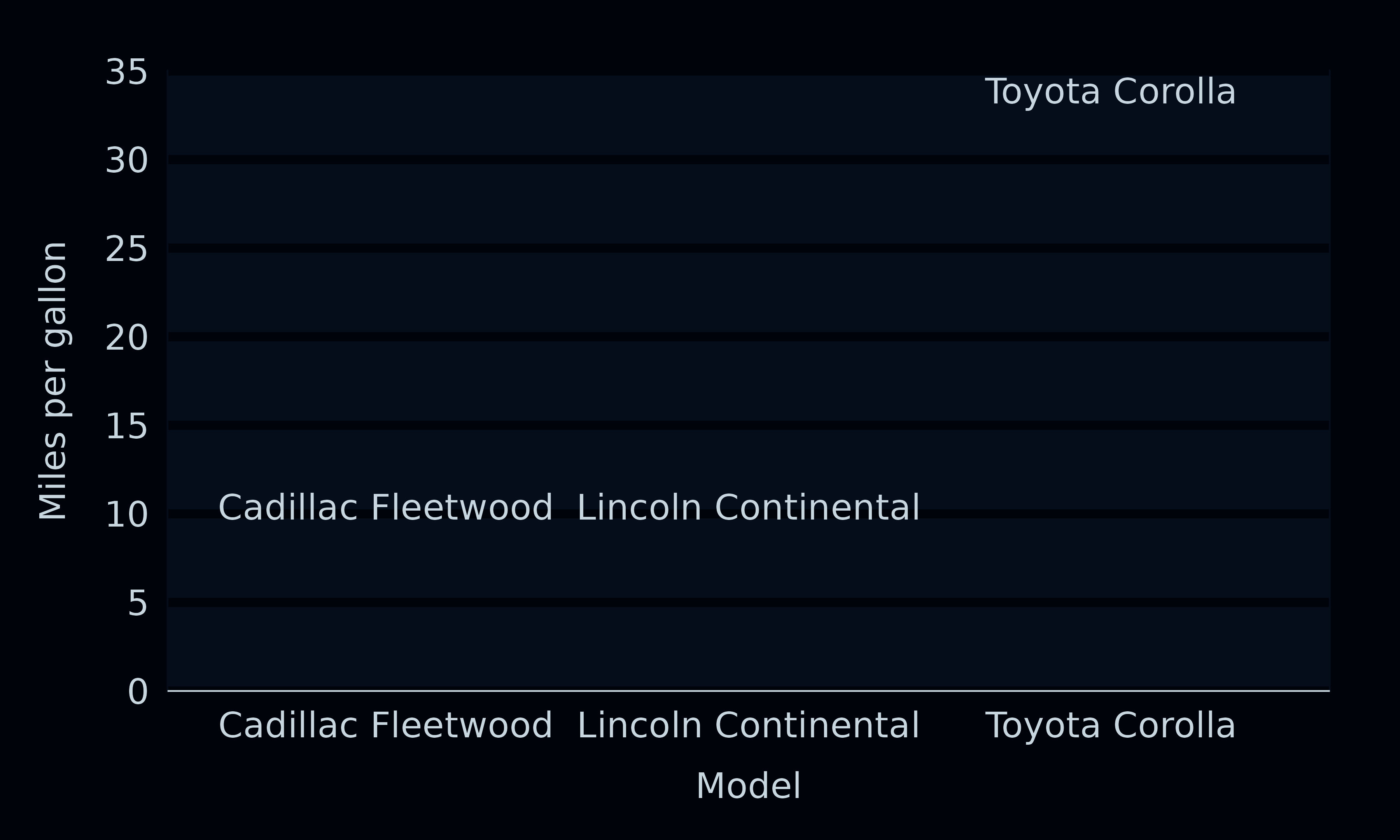
gg_text

bind_rows(
  mtcars |> slice_min(order_by = mpg),
  mtcars |> slice_max(order_by = mpg)) |>
  tibble::rownames_to_column("model") |>
  gg_text(
    x = model,
    y = mpg,
    label = model,
    y_expand_limits = 0,
    y_label = "Miles per gallon",
  )

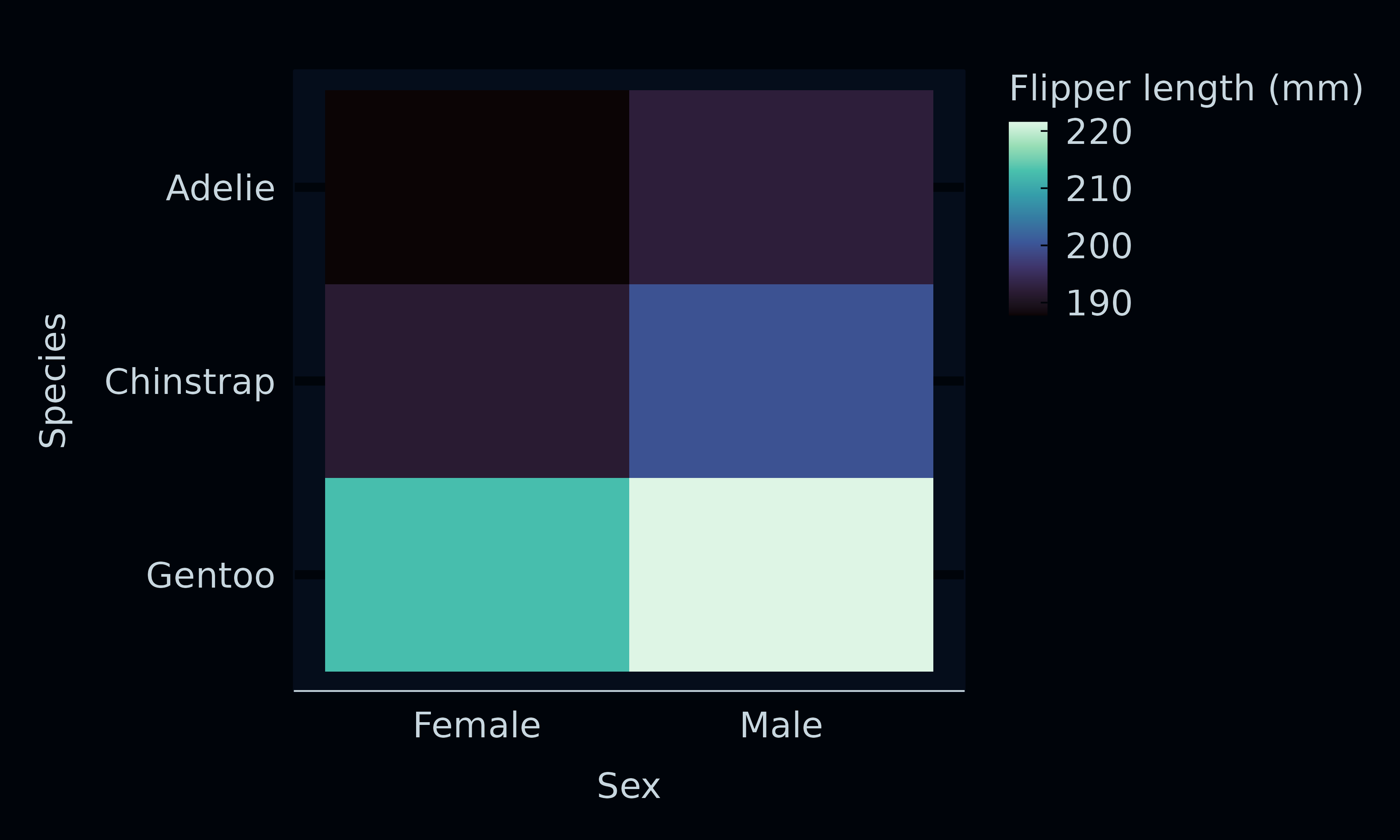
gg_tile

penguins2 |>
  group_by(species, sex) |>
  summarise(flipper_length_mm = mean(flipper_length_mm, na.rm = TRUE)) |>
  labelled::copy_labels_from(penguins2) |>
  gg_tile(
    x = sex,
    y = species,
    col = flipper_length_mm,
  )

gg_violin

penguins2 |>
  gg_violin(
    x = sex,
    y = body_mass_g,
    col = species,
  )

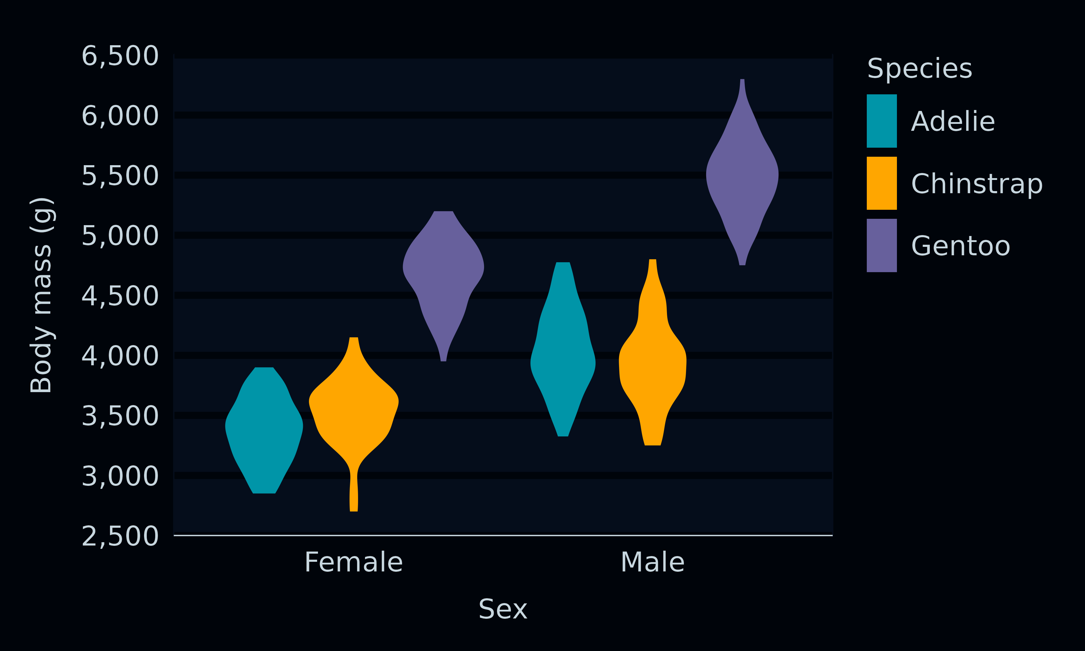
gg_blanket

penguins2 |>
  gg_blanket(
    geom = "violin",
    stat = "ydensity",
    position = "dodge",
    x = sex,
    y = body_mass_g,
    col = species,
  )