ggblanket

Overview

ggblanket is a package of ggplot2 wrapper functions.

The primary objective is to simplify ggplot2 visualisation.

Secondary objectives relate to:

Design: produce well-designed visualisation
Alignment: align with ggplot2 and tidyverse
Scope: cover much of what ggplot2 does.

Computational speed has been traded-off.

How it works

First setup with set_blanket()
Each gg_* function wraps a geom
A merged col argument to colour/fill by a variable
A facet argument to facet by a variable
A facet2 argument to facet by a 2nd variable
Other aesthetics via mapping argument
Prefixed arguments to customise x/y/col/facet
Smart *_label defaults for axis and legend titles
Other ggplot2::geom_* arguments via ...
Families of *_mode_* themes with legend variants
Side-effects to the mode based on the mode_orientation
One *_symmetric continuous scale
Ability to add multiple geom_* layers
Arguments to customise setup with set_blanket()
A gg_blanket() function with geom flexibility

library(dplyr)
library(stringr)
library(ggplot2)
library(scales)
library(ggblanket)
library(palmerpenguins)
library(patchwork)

penguins2 <- penguins |> 
  labelled::set_variable_labels(
    bill_length_mm = "Bill length (mm)",
    bill_depth_mm = "Bill depth (mm)",
    flipper_length_mm = "Flipper length (mm)",
    body_mass_g = "Body mass (g)",
  ) |> 
  mutate(sex = factor(sex, labels = c("Female", "Male"))) |> 
  tidyr::drop_na(sex)

1. First setup with `set_blanket()`

The set_blanket() function should be run first.

This sets the default style of plots with themes and colours etc. It can be customised.

It should be run at the start of every script or quarto document.

set_blanket()

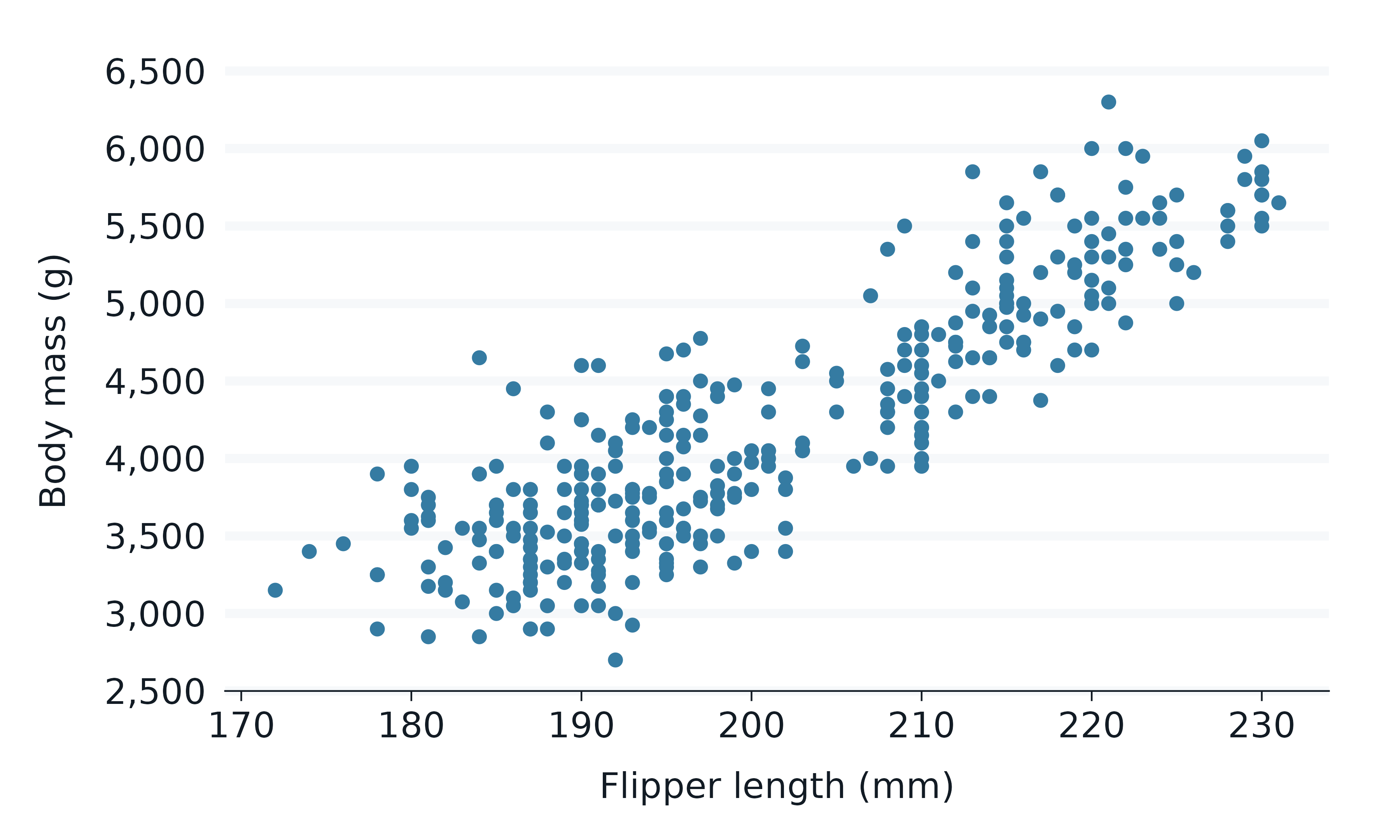
2. Each `gg_*` function wraps a geom

Each gg_* function wraps a ggplot2::ggplot() function with the associated ggplot2::geom_*() function.

Almost every geom in ggplot2 is wrapped.

Position related aesthetics can be added directly as arguments.

penguins2 |>
  gg_point(
    x = flipper_length_mm,
    y = body_mass_g,
  )

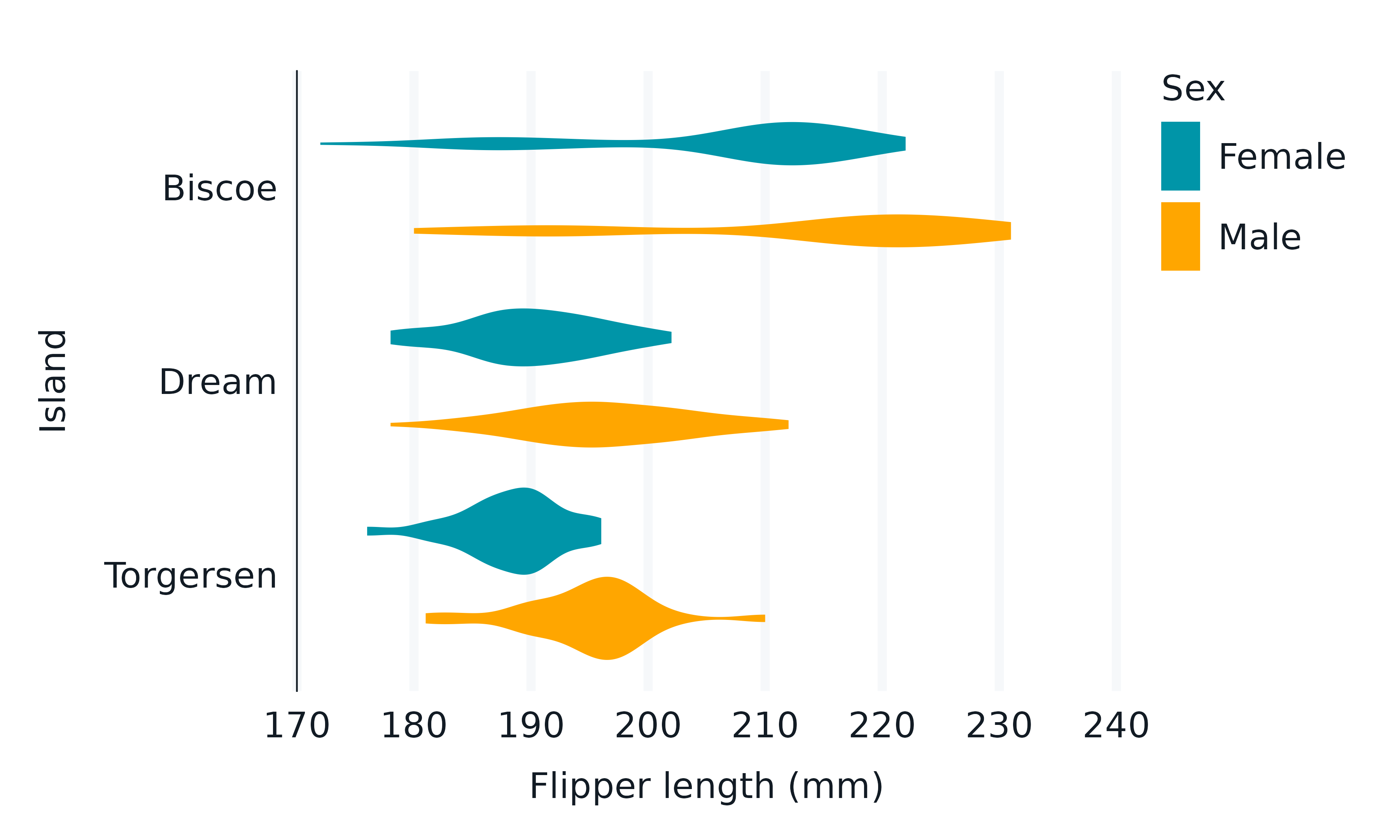
3. A merged `col` argument to colour/fill by a variable

The colour and fill aesthetics of ggplot2 are merged into a single concept represented by the col argument.

This combined aesthetic means that all colour outlines and all fill interiors should be coloured with the col_palette by the col variable.

Use colour = NA or fill = NA to turn one of these off.

penguins2 |>
  gg_boxplot(
    x = flipper_length_mm,
    y = island,
    col = sex, 
  )

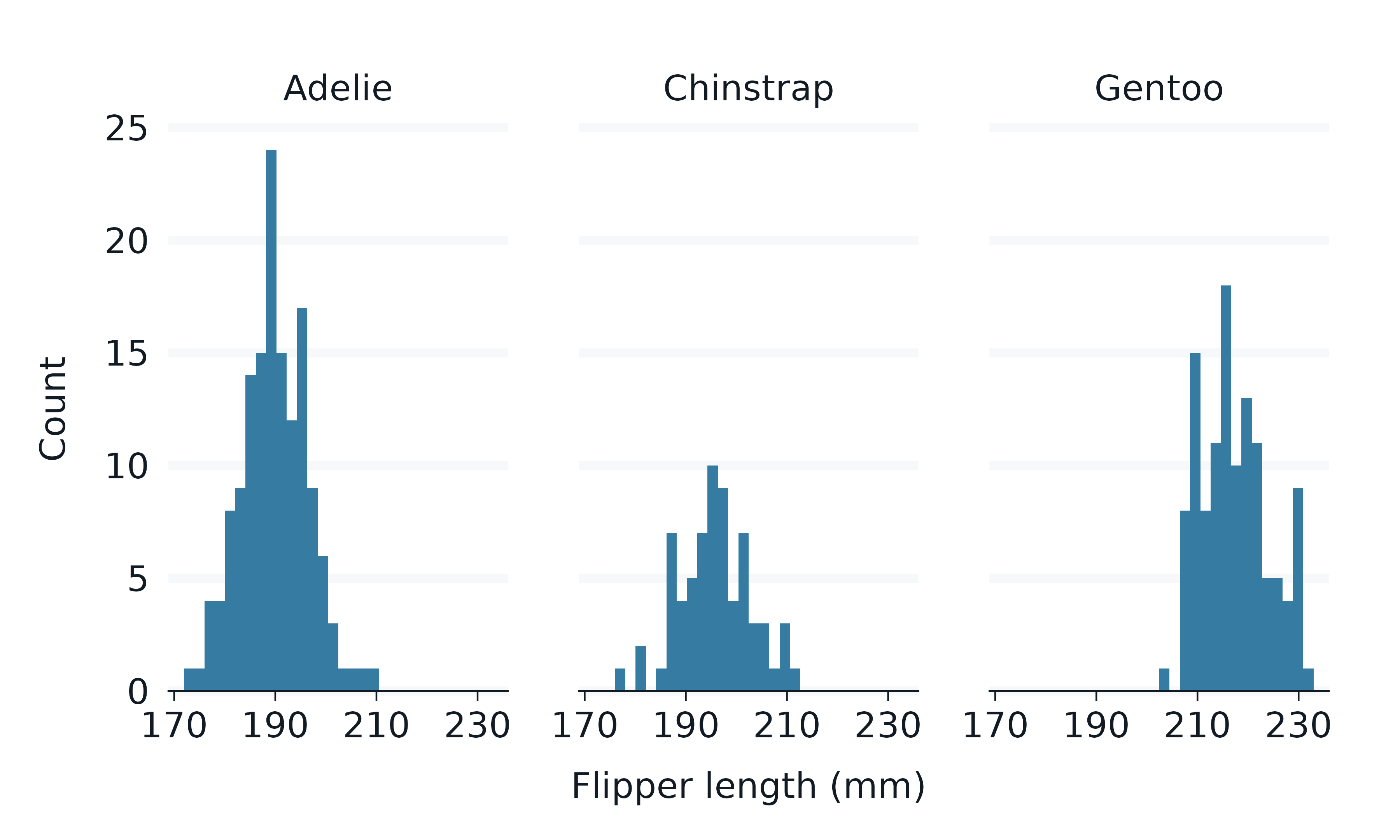
4. A `facet` argument to facet by a variable

Users provide an unquoted facet variable to facet by.

When facet is specified, the facet_layout will default to a "wrap" of the facet variable (if facet2 = NULL).

penguins2 |>
  gg_histogram(
    x = flipper_length_mm,
    facet = species,
  )

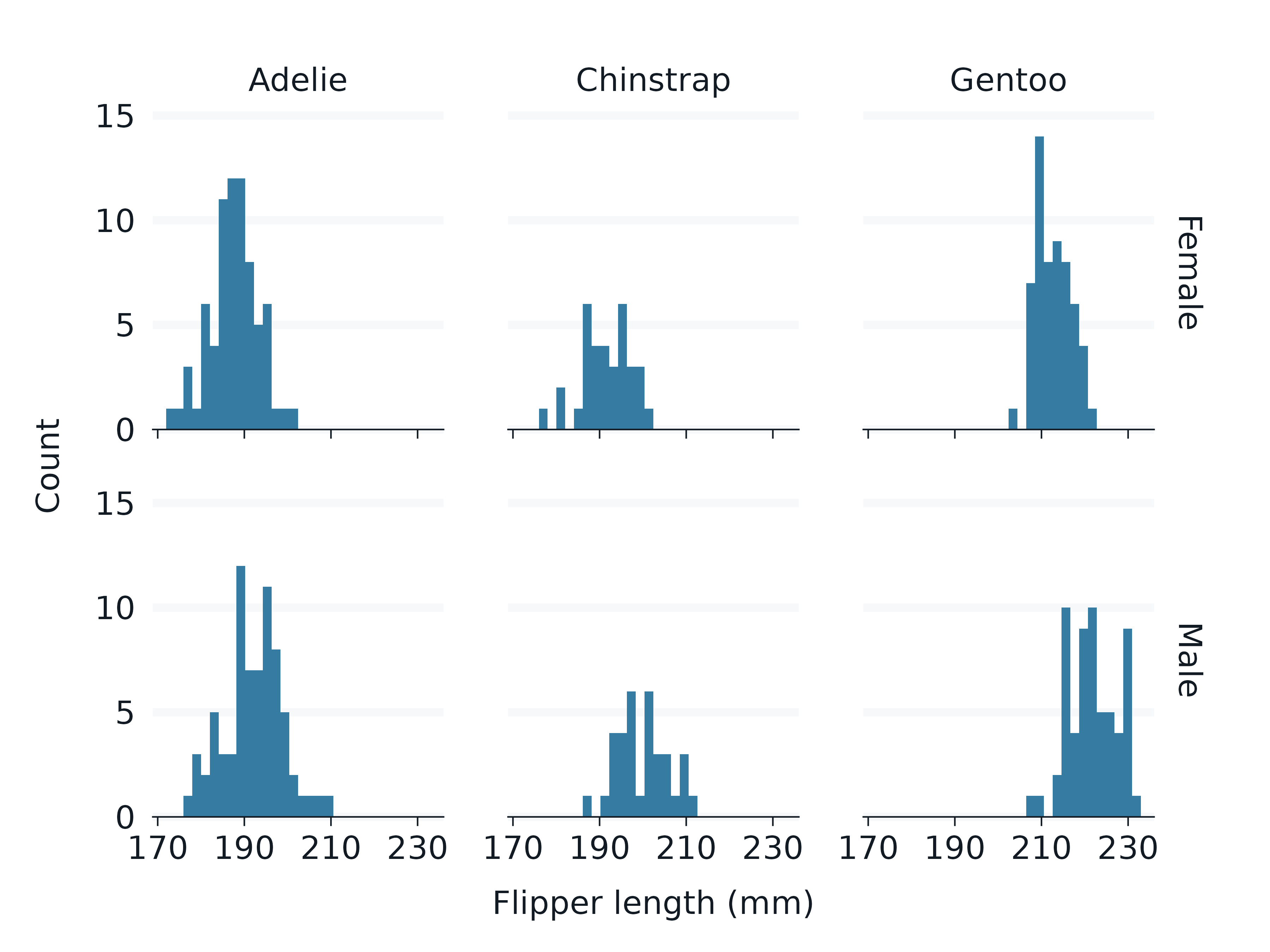
5. A `facet2` argument to facet by a 2nd variable

Users can also provide an unquoted facet2 variable to facet by.

When facet2 is specified, the facet_layout will default to a "grid" of the facet variable (horizontally) by the facet2 variable (vertically).

penguins2 |>
  gg_histogram(
    x = flipper_length_mm,
    facet = species,
    facet2 = sex,
  )

6. Other aesthetics via `mapping` argument

Some aesthetics are not available via an argument (e.g. alpha, size, shape, linetype and linewidth).

These can be accessed via the mapping argument using the aes() function.

To customise associated scales/guides, + on the applicable ggplot2 layer. In some situations, you may need to override the colour used in the guide, or reverse the values in the relevant scale etc.

The mapping argument can also be used to add only a colour or fill aesthetic scale, and not both.

penguins2 |> 
  gg_jitter(
    x = species, 
    y = flipper_length_mm, 
    col = island,
    mapping = aes(shape = sex),
  ) +
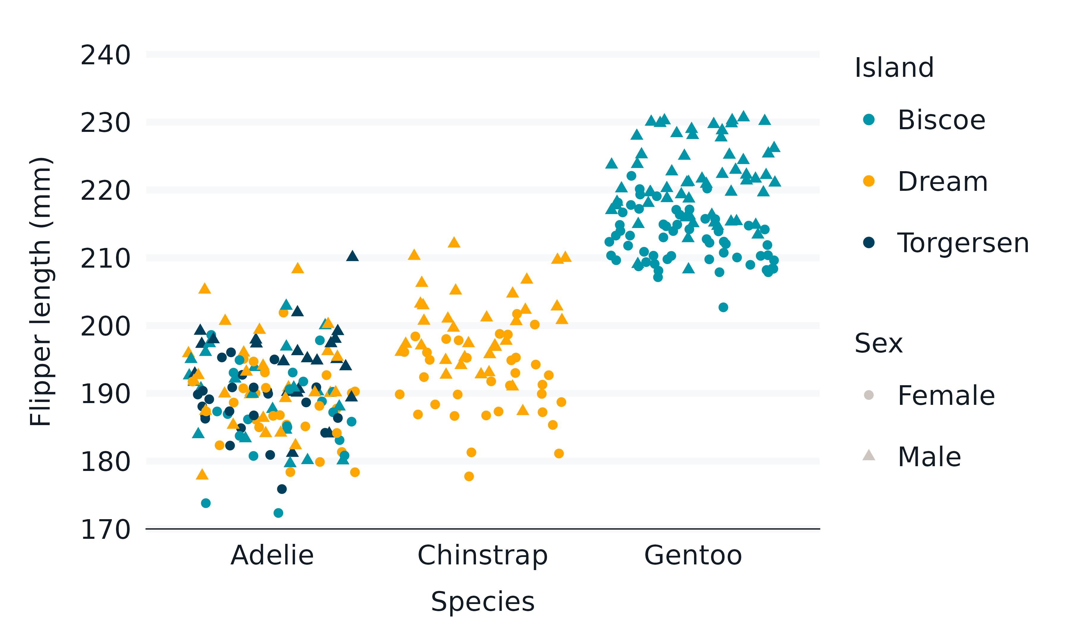
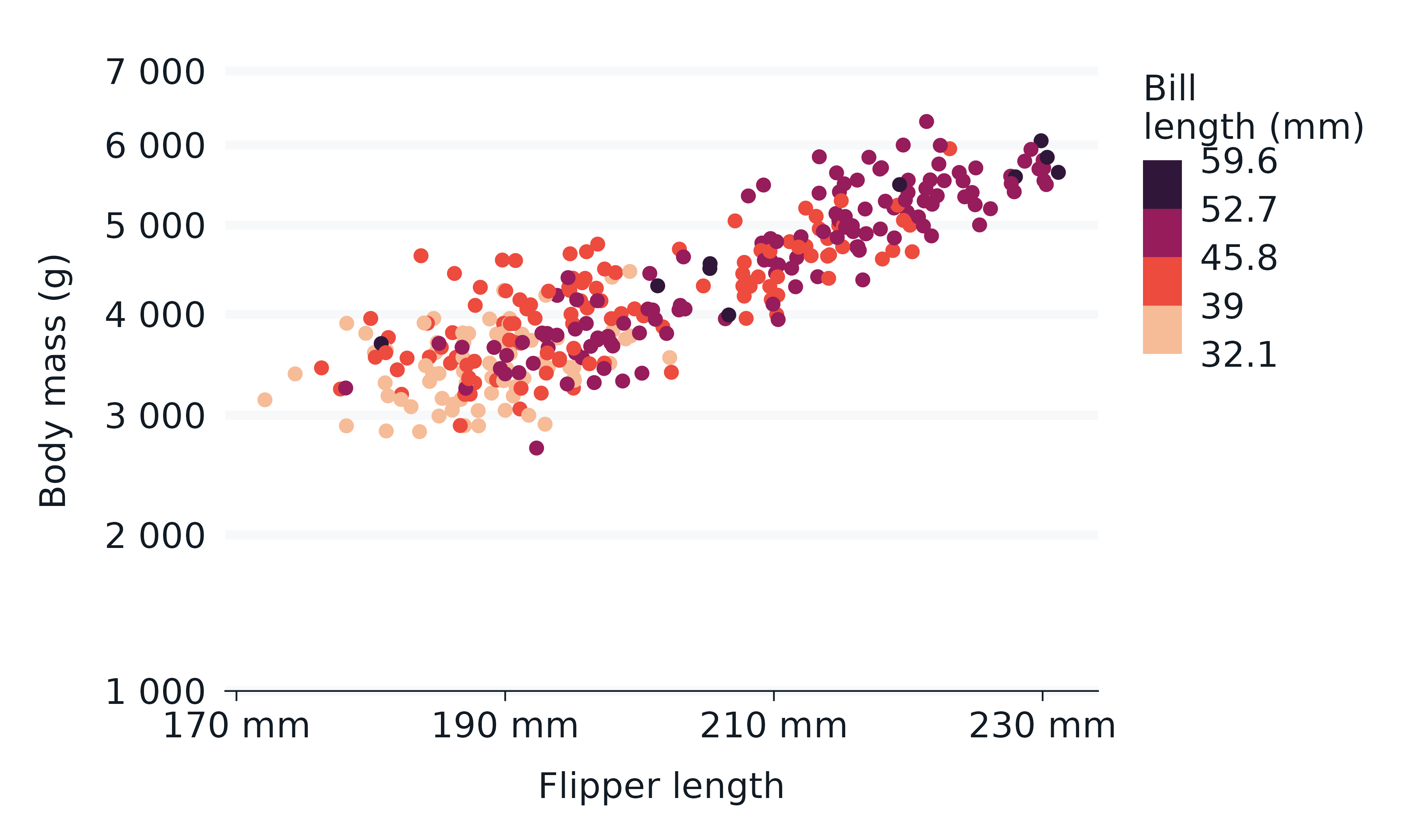
  guides(shape = guide_legend(override.aes = list(colour = grey)))

7. Prefixed arguments to customise x/y/col/facet

There are numerous arguments to customise plots that are prefixed by whether they relate to x, y, col or facet.

For x, y and col, these relate to associated arguments within ggplot2 scales and guides. For facet, they relate to associated arguments within ggplot2::facet_wrap and ggplot2::facet_grid.

Scales and guides associated with other other aesthetics can be customised by adding the applicable ggplot2 layer.

penguins2 |>
  gg_jitter(
    x = flipper_length_mm,
    y = body_mass_g,
    col = flipper_length_mm,
    x_breaks_n = 4,
    x_labels = \(x) stringr::str_sub(x, 1, 1),
    y_expand_limits = 1000,
    y_labels = label_number(big.mark = " "), 
    y_transform = "sqrt",
    col_label = "Flipper\nlength (mm)",
    col_steps = TRUE,
    col_breaks = \(x) quantile(x, seq(0, 1, 0.25)),
    col_palette = viridis::rocket(n = 9, direction = -1),
  )

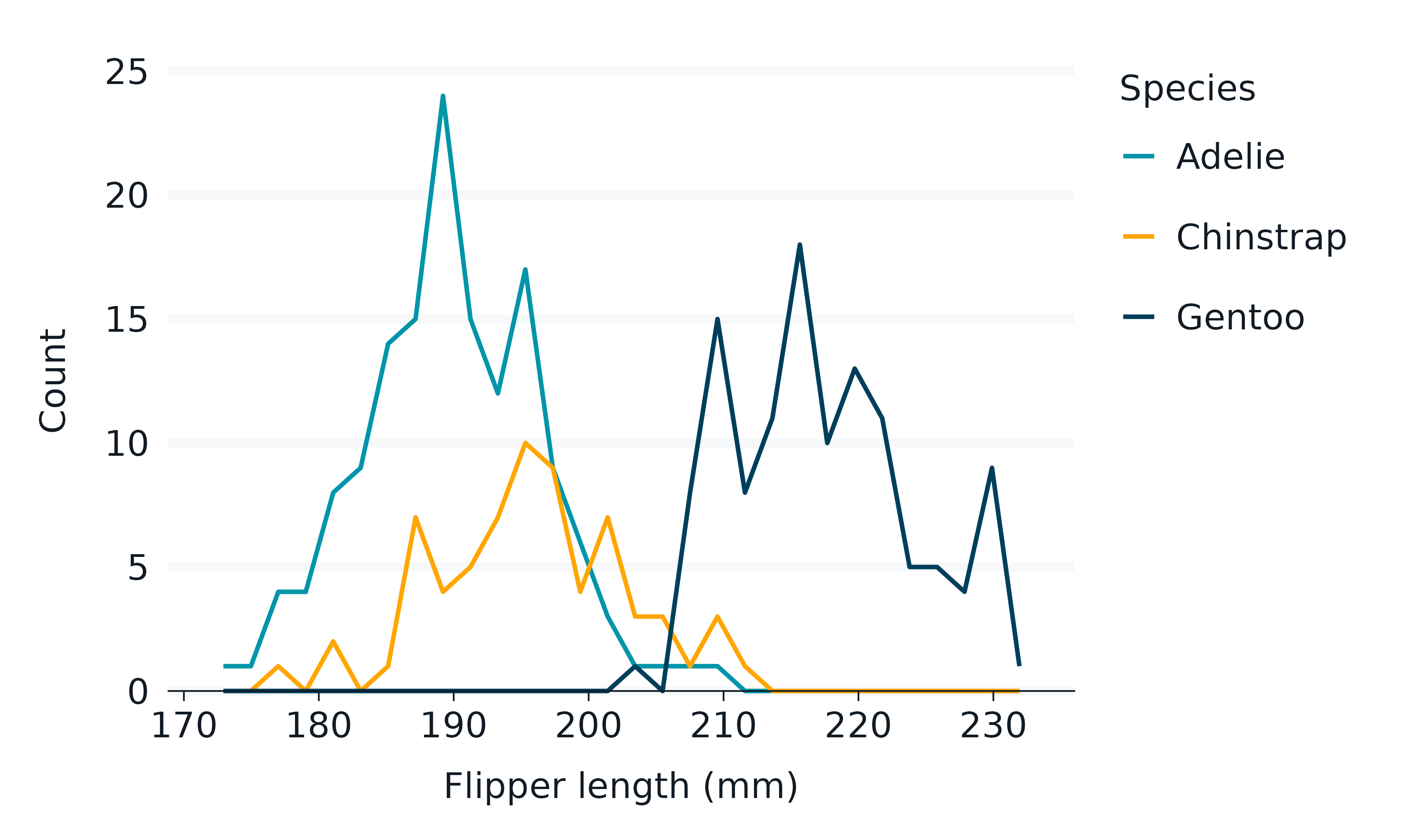
8. Smart `*_label` defaults for axis and legend titles

The x_label, y_label and col_label for the axis and legend titles can be manually specified with the applicable *_label argument (or + ggplot2::labs(...)).

If not specified, they will first take any label attribute associated with the applicable variable.

If none, they will then convert the variable name to a label name using the label_to_case function, which defaults to sentence case (i.e. snakecase::to_sentence_case).

penguins2 |>
  gg_freqpoly(
    x = flipper_length_mm,
    col = species,
  )

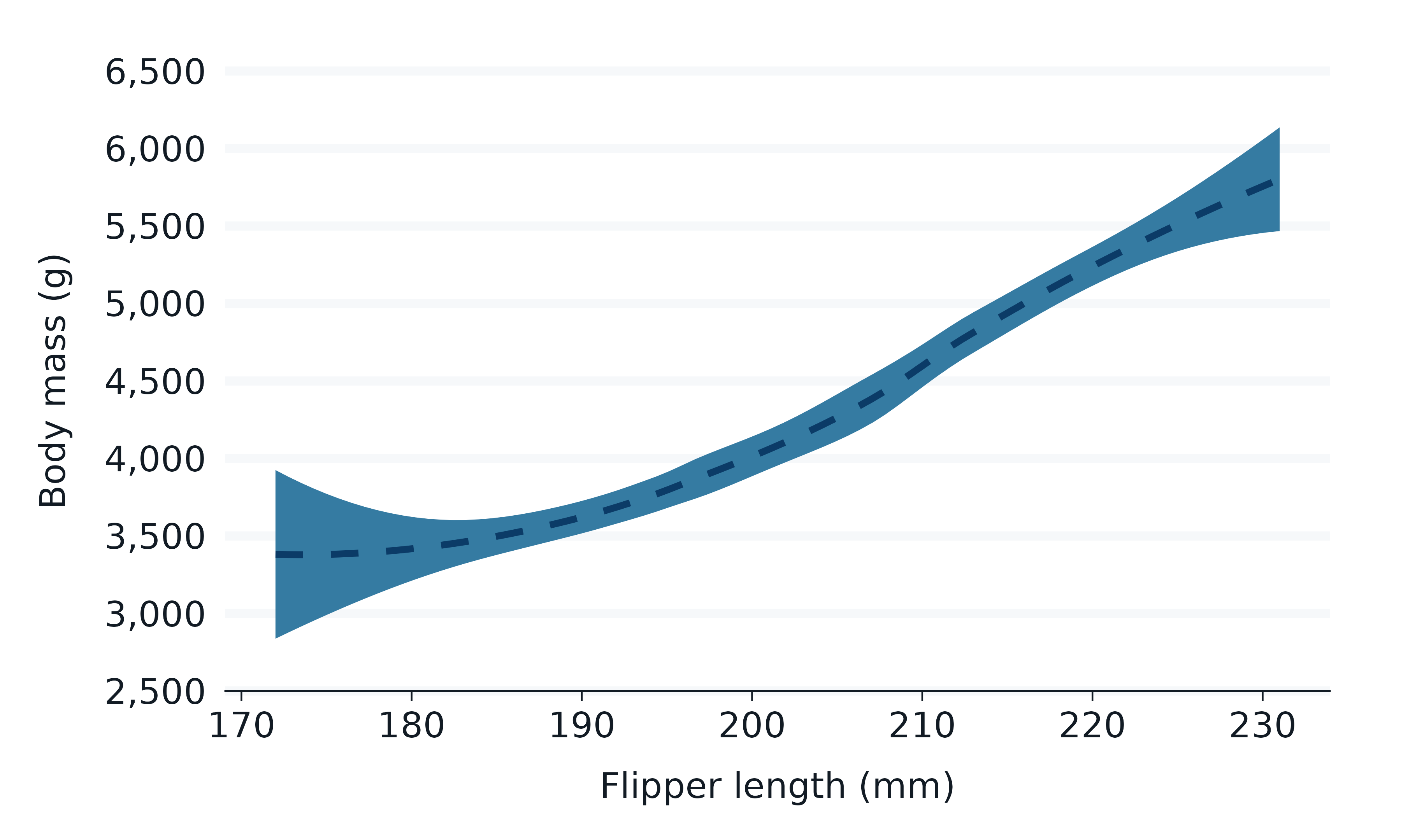
9. Other `ggplot2::geom_*` arguments via `...`

The ... argument provides access to all other arguments in the ggplot2::geom_*() function.

Common arguments to add include colour, fill, alpha, linewidth, linetype, size and width, which enables fixing of these to a particular value.

Use the ggplot2::geom_* help to see what arguments are available.

penguins2 |>
  gg_smooth(
    x = flipper_length_mm,
    y = body_mass_g,
    col = sex, 
    col_palette = c("#003F5CFF", "#FFA600FF"),
    colour = "#BC5090FF", 
    linewidth = 1, 
    linetype = "dashed",
    alpha = 1, 
    se = TRUE, 
    level = 0.999, 
  )

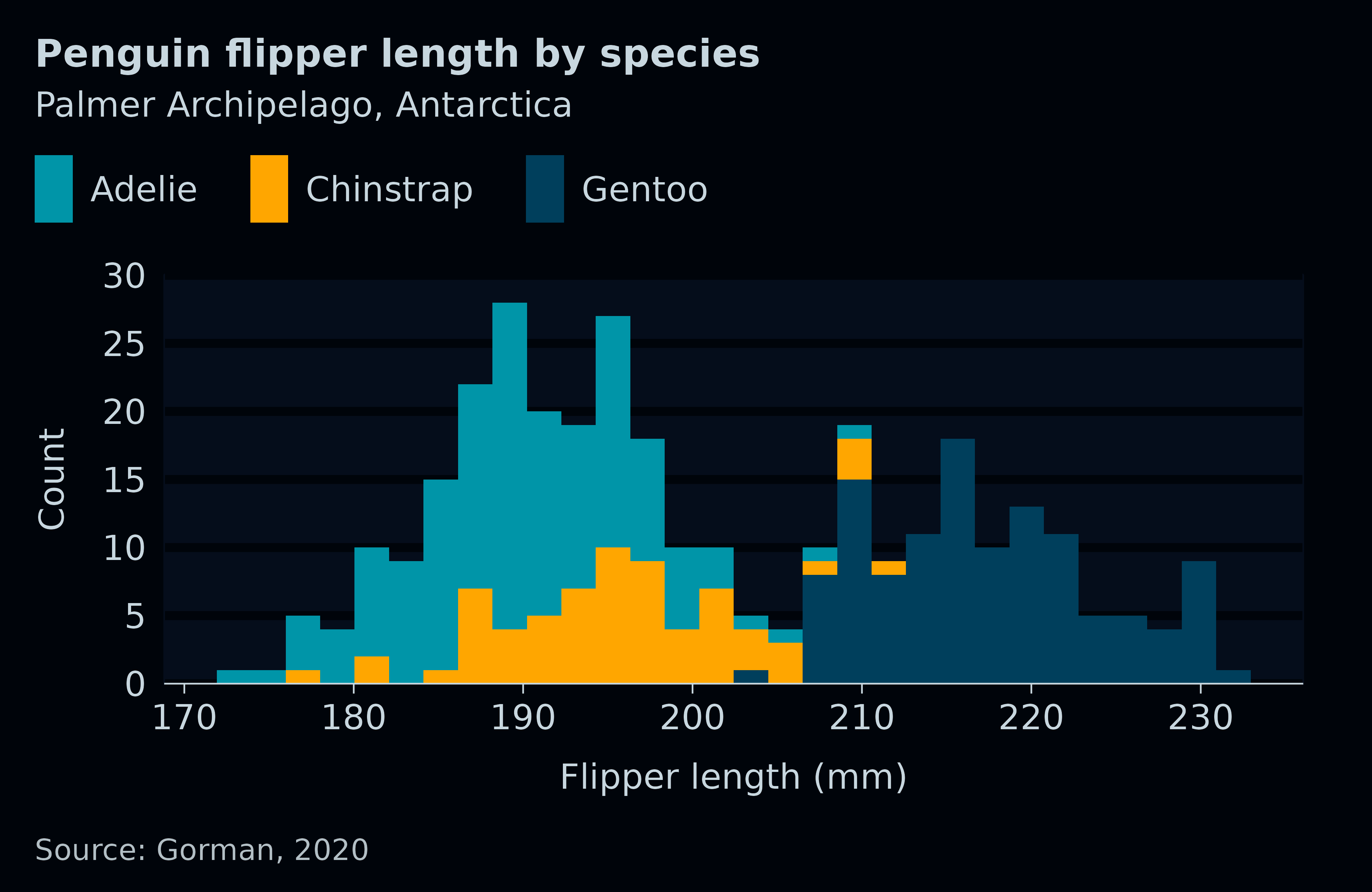
10. Families of `_mode_` themes with legend variants

light_mode_* and dark_mode_* theme families are provided with variants that differ based on legend placement with suffix r (right), b (bottom), and t (top). These functions were built for use with the mode argument - and have flexibility to adjust colours, linewidths etc.

penguins2 |>
  gg_histogram(
    x = flipper_length_mm,
    col = species,
    title = "Penguin flipper length by species",
    subtitle = "Palmer Archipelago, Antarctica",
    caption = "Source: Gorman, 2020", 
    mode = dark_mode_t() + theme(legend.title = element_blank()),
  )

11. Side-effects to the `mode` based on the `mode_orientation`

The gg_* function adds helpful side-effects to the mode.

Where mode_orientation = "x", the gg_* function will remove the y axis line/ticks and the x gridlines from the mode (by changing their colour to “transparent”). Where it is mode_orientation = "y", the opposite will occur. If the gg_* guesses an incorrect mode_orientation, then the user can change this.

Additionally, the gg_* function will remove ticks from discrete scales.

Any mode used should be designed to anticipate these side-effects. To avoid these side-effects, instead + the theme on to the gg_* output (or use the theme argument in set_blanket).

p1 <- penguins2 |>
  gg_jitter(
    x = sex,
    y = bill_depth_mm,
  )

p2 <- penguins2 |>
  gg_jitter(
    x = bill_depth_mm,
    y = sex,
  ) 

p1 + p2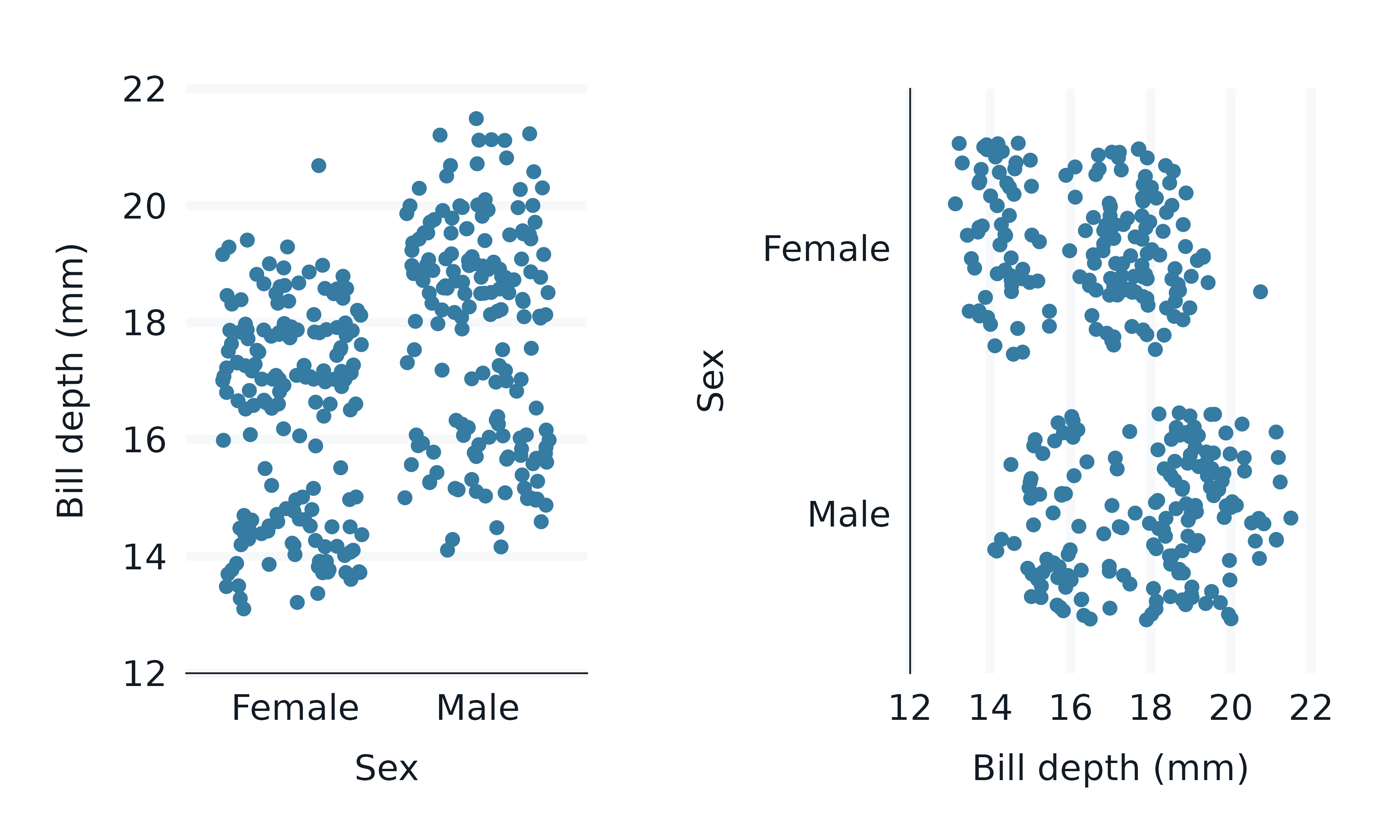

12. One `*_symmetric` continuous scale

One *_symmetric continuous scale can be made where:

*_transform is linear
the stat is not “sf”
if faceted, the relevant scale is fixed

By default, the gg_* function will make a x_symmetric scale if there is a y discrete axis and a x continuous axis. Otherwise, it will make a y_symmetric scale.

A y_symmetric axis makes:

the limits locked to the range of the y_breaks
the y_expand default to c(0, 0).

The vice versa occurs for an x_symmetric axis.

Use *_symmetric = FALSE to revert to the normal limits and expand defaults (i.e. the limits of the range of the data including *_expand_limits with *_expand = c(0.05, 0.05)).

Note all continuous scales ensure all data is kept using scales::oob_keep - and, by default, are left unclipped (i.e. coord_cartesian(clip = "off").

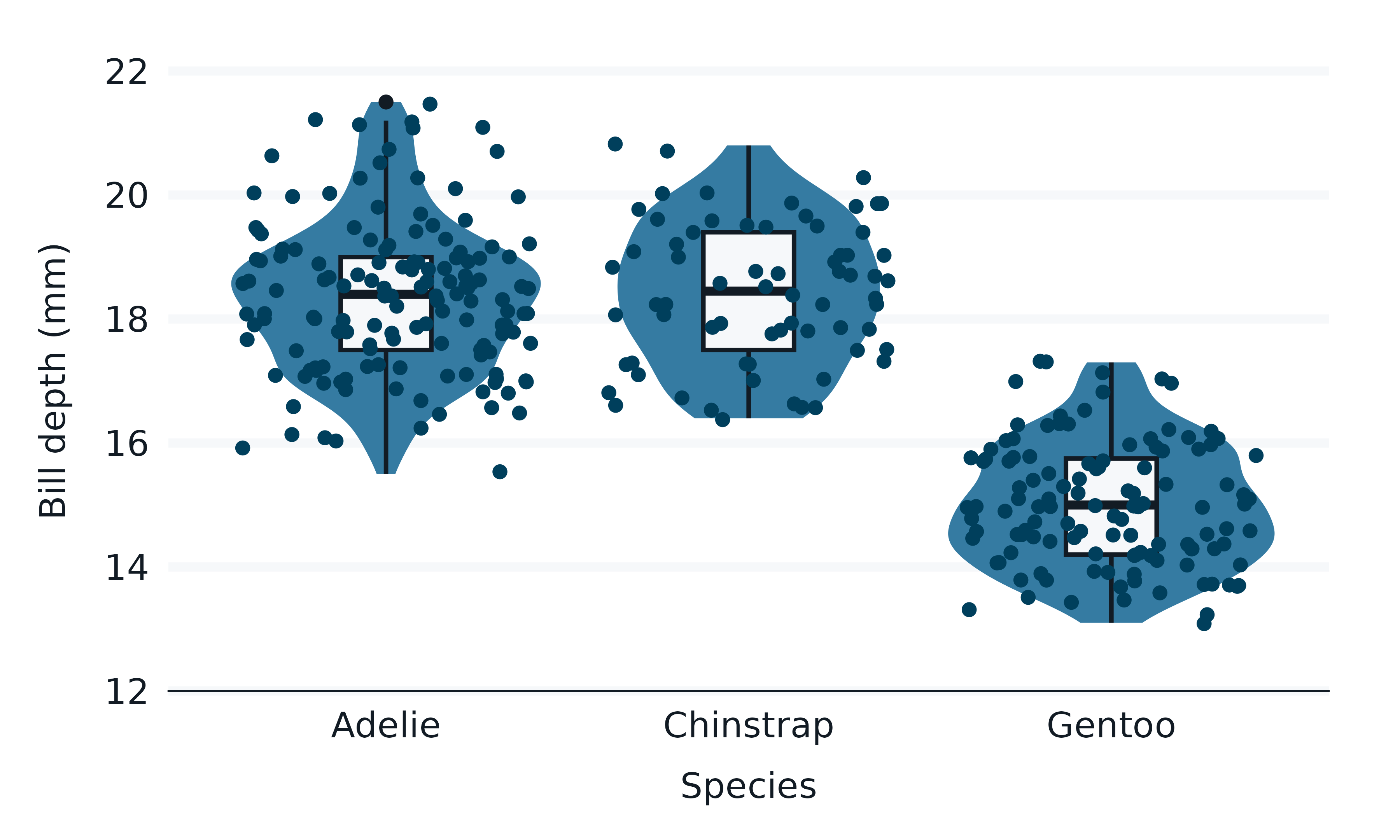
13. Ability to add multiple `geom_*` layers

Users can make plots with multiple ggplot2::geom_* layers.

The gg_*() geom layer will be the bottom geom layer of the plot, and each subsequent geom_*() layer is placed on top.

Aesthetics added directly (e.g. x, y etc.) to the gg_*() function will inherit to later geom_*() layers, whereas those added to the mapping argument will not.

penguins2 |> 
  gg_violin(
    x = species, 
    y = bill_depth_mm,
    outliers = FALSE,
  ) +
  geom_boxplot(
    width = 0.25,
    colour = lightness[1],
    fill = lightness[2],
  ) +
  geom_jitter(
    colour = navy,
  )

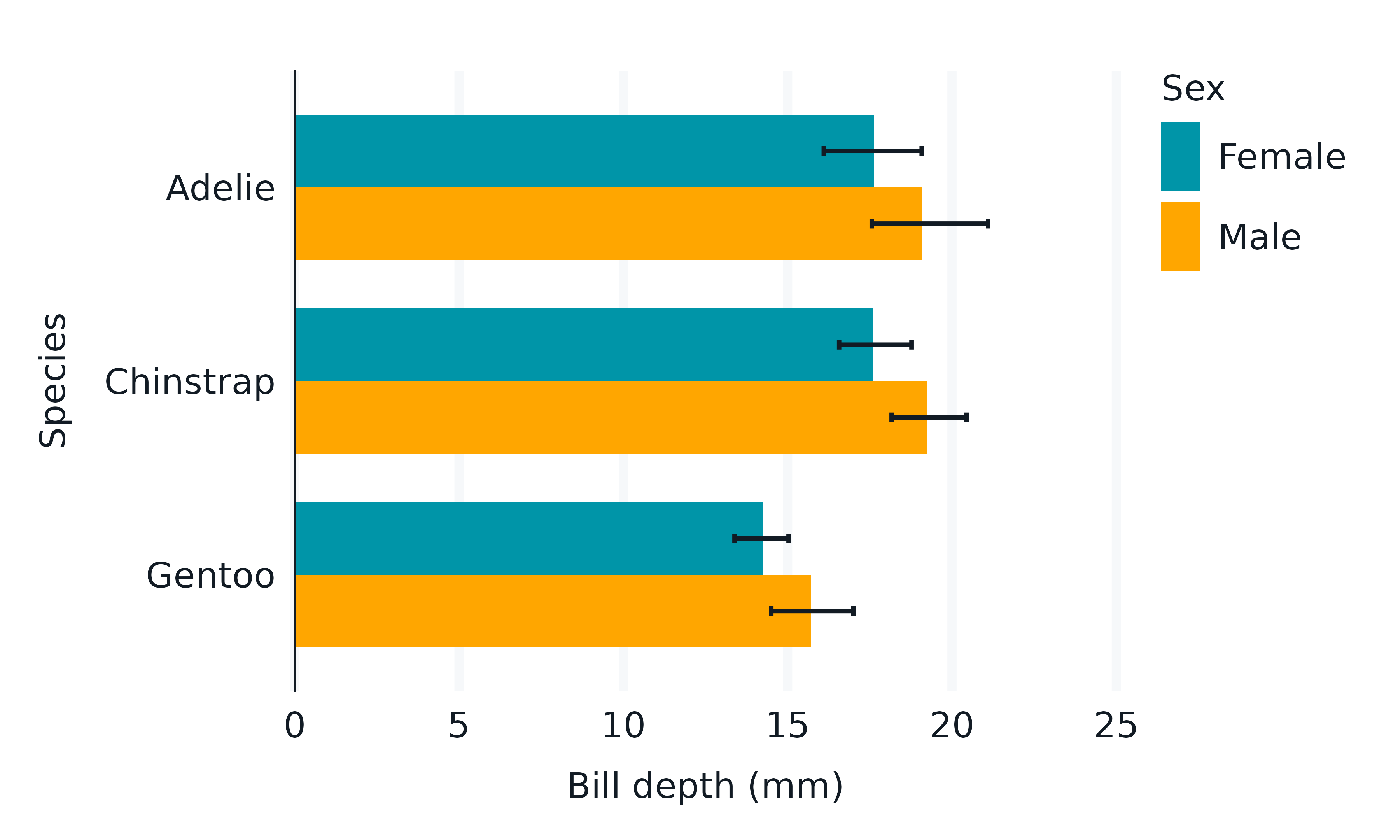
The scales are built within the gg_*() function without knowledge of later layers. The gg_*() function builds scales with regard to the stat, position, and aesthetics (that the geom understands) etc. So, in some situations, users will need to take care.

penguins2 |>
  group_by(species, sex) |>
  summarise(
    lower = quantile(bill_depth_mm, probs = 0.05),
    upper = quantile(bill_depth_mm, probs = 0.95),
    bill_depth_mm = mean(bill_depth_mm, na.rm = TRUE),
  ) |>
  labelled::copy_labels_from(penguins2) |>
  gg_blanket(
    y = species,
    x = bill_depth_mm,
    xmin = lower, 
    xmax = upper,
    col = sex,
    position = position_dodge(width = 0.75),
    x_expand_limits = 0,
  ) +
  geom_col(
    width = 0.75,
    position = position_dodge(width = 0.75),
    alpha = 0.9,
  ) +
  geom_errorbar(
    width = 0.1, 
    position = position_dodge(width = 0.75),
    colour = lightness[1],
  )

14. Arguments to customise setup with `set_blanket()`

The set_blanket function sets customisable defaults for the:

mode (i.e. a theme added with side-effects)
geom defaults (i.e. colour/fill used where no colour aesthetic scale)
discrete colour palette (and NA colour)
continuous colour palette (and NA colour)
theme (i.e. a theme added with no side-effects)

The ggplot2::update_geom_defaults() function can be used to further fine-tune geom defaults.

set_blanket() also works on ggplot2 code.

set_blanket(
  mode = dark_mode_r(), 
  colour = "#E7298AFF",
  colour_text = darkness[1],
  col_palette_d = c("#1B9E77FF", "#D95F02FF", "#7570b3FF", "#E7298AFF", "#66A61EFF", 
                    "#E6AB02FF", "#A6761DFF", "#666666FF"), #RColorBrewer Dark2 
)

p1 <- penguins2 |>
  gg_point(
    x = flipper_length_mm, 
    y = body_mass_g,
    x_breaks_n = 4, 
  ) +
  geom_vline(xintercept = 200) +
  annotate("text", x = I(0.25), y = I(0.75), label = "Here")

p2 <- penguins2 |> 
  gg_histogram(
    x = flipper_length_mm,
    col = species,
    x_breaks_n = 4, 
  ) +
  geom_vline(xintercept = 200) +
  annotate("text", x = I(0.75), y = I(0.75), label = "Here")

p1 + p2


set_blanket()

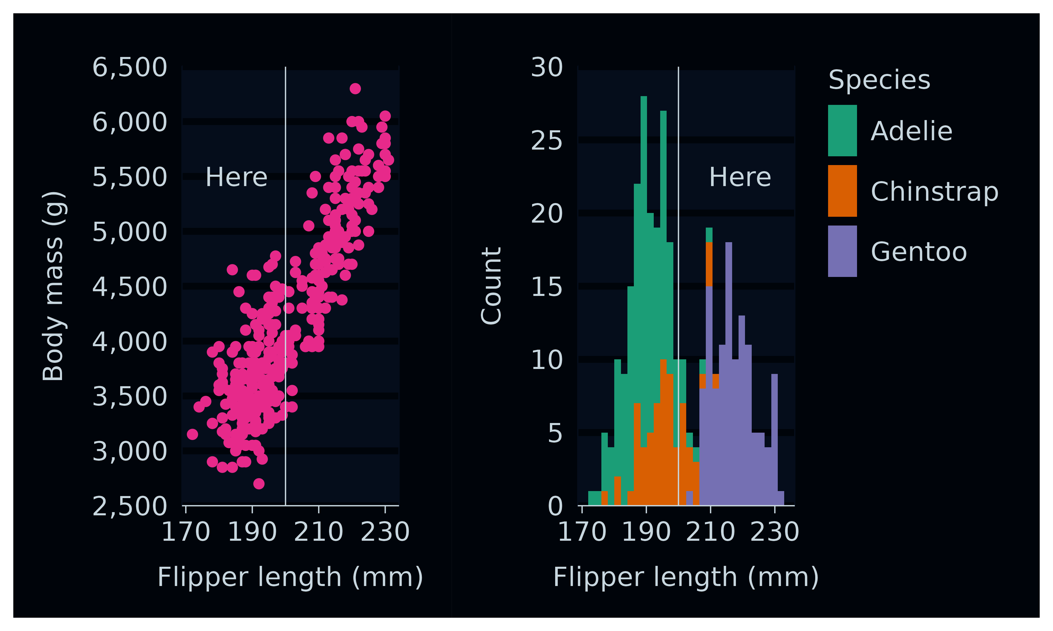
15. A `gg_blanket()` function with `geom` flexibility

The package is driven by the gg_blanket function, which has a geom argument with ggplot2::geom_blank defaults for geom, stat and position.

All other functions wrap this function with a fixed geom, and their own default stat and position arguments as per the applicable geom_* function.

This function can often be used with geoms that do not have an associated gg_* function.

geom_spoke()
#> geom_spoke: na.rm = FALSE
#> stat_identity: na.rm = FALSE
#> position_identity

expand.grid(x = 1:10, y = 1:10) |>
  tibble() |>
  mutate(angle = runif(100, 0, 2*pi)) |>
  mutate(speed = runif(100, 0, sqrt(0.1 * x))) |>
  gg_blanket(
    geom = "spoke",
    x = x, 
    y = y,
    col = speed,
    mapping = aes(angle = angle, radius = speed),
  ) +
  geom_point()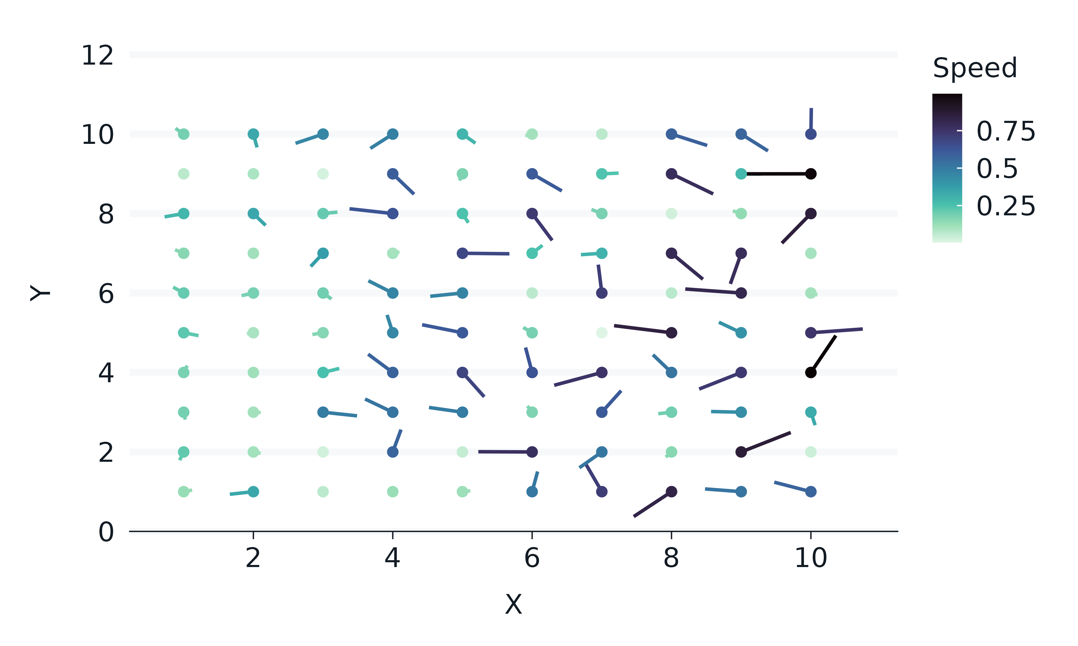

Further information

See the ggblanket website for further information, including articles and function reference.

David Hodge

Overview

How it works

1. First setup with set_blanket()

2. Each gg_* function wraps a geom

3. A merged col argument to colour/fill by a variable

4. A facet argument to facet by a variable

5. A facet2 argument to facet by a 2nd variable

6. Other aesthetics via mapping argument

7. Prefixed arguments to customise x/y/col/facet

8. Smart *_label defaults for axis and legend titles

9. Other ggplot2::geom_* arguments via ...

10. Families of *_mode_* themes with legend variants

11. Side-effects to the mode based on the mode_orientation

12. One *_symmetric continuous scale

13. Ability to add multiple geom_* layers

14. Arguments to customise setup with set_blanket()

15. A gg_blanket() function with geom flexibility